
Rapid ship detection in remote sensing images based on visual saliency model
-
摘要: 为了降低传统高分辨率海面遥感图像舰船目标检测方法的计算复杂度,提高检测速度,在舰船目标检测中引入了基于直方图对比度的视觉显著模型和空间降维算法,提出一种新的高分辨率海面遥感图像舰船目标快速检测算法。首先对高分辨率遥感图像进行空间降维,然后计算降维图的视觉显著图,突出感兴趣目标区域,最后利用最大类间方差法分割视觉显著图以获取舰船目标候选区域。结果表明,目标检测所消耗的时间减小为原来的10%~12%,弱化了复杂海面纹理背景对目标检测的影响。该研究提高了高分辨率遥感图像舰船目标的检测效率。Abstract: In order to reduce the computational complexity of ship target detection methods for sea surface remote sensing images of traditional high resolution and improve the speed of detection, combined with visual salience algorithm based on histogram contrast and spatial dimension reduction algorithm, a new ship target fast detection algorithm for sea surface remote sensing images of high resolution was proposed.Firstly, spatial dimension reduction of high resolution remote sensing images was carried out. The saliency map was calculated and the interest area of the target area was highlighted. At last, the visual salient image was segmented by the method of maximum inter class variance to obtain the candidate region of the ship target. The results show that the time consumed by the target detection is reduced to 10%~12% of the original.The influence of complex sea surface texture background on target detection is weakened.The research improves ship target detection efficiency for high resolution remote sensing images.
-
Keywords:
- image processing /
- ship detection /
- visual salience /
- spatial dimension reduction /
- remote sensing
-
引言
随机共振现象是噪声和非线性动力学相互作用出现的一种有趣的现象。1981年被BENZI等人首次发现,此后在很多领域成为人们广泛研究的课题,在实验和理论研究上都取得了很大的进展。但是现有的研究成果大多受限于单一频率的周期驱动信号。而在实践应用中,需要使载波振幅按照调制信号的改变而实行调制,使其保持着高频载波的频率特性, 需要将此调制信号加载到激光源上,使其作为传递信息的工具。这对激光通讯和提高激光的效率有重要的作用。通常,传统的随机共振一般由信噪比与噪声强度的关系来体现。1998年,BARZYKIN等人提出可以用信噪比与噪声自相关时间的关系来体现。CHENG等人用信噪比与净增益系数之间的变化关系也阐明了这点。后来的研究说明了随机共振可由信噪比与系统中其它参量之间的关系来体现。作者用线性化近似方法计算了在偏置调幅信号下,色抽运噪声和实部、虚部间关联的量子噪声驱动的单模激光损失模型的输出光强信噪比,发现信噪比与系统的净增益系数之间存在共振现象。此外,还讨论了输入信号和噪声在量子噪声实部虚部间弱关联和强关联时对随机共振的影响,为优化激光系统的动力学性质提供依据。
1. 输入偏置调幅波的单模激光损失模型的光强关联函数及信噪比
单模激光损失模型输入偏置调幅波后的光强方程为:
dIdt′=2a0I−2AI2+Q (1−|λ|)+2Ipr(t′)+2√Iεr(t′)+B[1−Dcos(Ωt′)]cos(ωt′) (1) 抽运噪声p(t′)和量子噪声ε(t′)的统计性质为:
{⟨pr(t′)⟩=⟨εr(t′)⟩=0⟨pr (t) pr(t′)⟩=P2τexp(|t−t′|τ)⟨εr(t)εr(t′)⟩=Q (1+|λ|)δ(t−t′)⟨pr(t)εe(t′)⟩=⟨pr(t′)εr(t)⟩=0 (2) 式中,a0为净增益系数, A为自饱和系数; I为光强, B为载波信号振幅,Ω为低频调制信号频率;pr(t′)为抽运噪声实部, εr(t′)为位相锁定后的量子噪声;P和Q是抽运噪声强度和量子噪声强度, τ为抽运噪声自关联时间, ω为高频载波信号频率, D为调制信号振幅;λ为量子噪声实部、虚部之间的关联系数,其取值范围为λ≤1。本文中所讨论的物理量,均无量纲。
设I=I0+δ(t′),δ(t′)为微小扰动项,I0为定态光强。在I0=a0/A附近, 对(1)式线性化处理得:
dδ(t′)/dt′=−γδ(t′)+Q (1−|λ|)+2I0pr(t′)+2√I0εr(t′)+B[1−Dcos(Ωt′)]cos(ωt′) (3) 式中, γ=2a0。
定义归一化稳态平均光强关联函数:
C(t)=lim (4) 进行傅里叶变换, 得出光强的功率谱:
S\text{ }\left( \omega ' \right)={{S}_{1}}\left( \omega ' \right)+{{S}_{2}}\left( \omega ' \right) 式中, S1(ω′)为输出信号功率谱, S2(ω′)为输出噪声功率谱。输出信号功率谱中有3个信号频率,输出总信号功率为:
{{P}_{S}}=\int_{0}^{\infty }{{{S}_{1}}(\omega ')\text{ d}\omega '} (5) 信噪比的定义为输出信号功率与3个信号频率处单位噪声功率之和的比值(只取正ω的谱):
R=\frac{{{P}_{S}}}{{{S}_{2}}\left( \omega \right)+{{S}_{2}}\left( \omega +\mathit{\Omega } \right)+{{S}_{2}}(\omega -\mathit{\Omega })} (6) 式中,
\begin{matrix} {{P}_{S}}=\frac{{{\text{ }\!\!\pi\!\!\text{ }}^{2}}{{B}^{2}}{{D}^{2}}}{4{{I}_{0}}^{2}{{\left[ {{\gamma }^{2}}+{{\left( \mathit{\Omega }+\omega \right)}^{2}} \right]}^{2}}}\left[ \frac{{{\gamma }^{2}}}{\mathit{\Omega }+\omega }+\left( \mathit{\Omega }+\omega \right) \right]+ \\ \frac{{{\text{ }\!\!\pi\!\!\text{ }}^{2}}{{B}^{2}}{{D}^{2}}}{4{{I}_{0}}^{2}{{\left[ {{\gamma }^{2}}+{{\left( \mathit{\Omega }-\omega \right)}^{2}} \right]}^{2}}}\left[ \frac{{{\gamma }^{2}}}{\mathit{\Omega }-\omega }+\left( \mathit{\Omega }-\omega \right) \right]+\frac{{{\text{ }\!\!\pi\!\!\text{ }}^{2}}{{B}^{2}}}{{{I}_{0}}^{2}\Omega ({{\gamma }^{2}}+{{\omega }^{2}})} \\ \end{matrix} (7) \left\{ \begin{align} &{{S}_{2}}\left( \omega \right)=\frac{2\text{ }\!\!\pi\!\!\text{ }{{Q}^{2}}{{\left( 1-\left| \lambda \right| \right)}^{2}}}{{{I}_{0}}^{2}{{\gamma }^{2}}}+\frac{4P{{\tau }^{2}}}{({{\gamma }^{2}}{{\tau }^{2}}-1)({{\omega }^{2}}{{\tau }^{2}}+1)}+ \\ &\frac{4}{{{\gamma }^{2}}+{{\omega }^{2}}}\left[ \frac{Q\text{ }\left( 1+\left| \lambda \right| \right)}{{{I}_{0}}}-\frac{P}{{{\gamma }^{2}}{{\tau }^{2}}-1} \right] \\ &{{S}_{2}}\left( \omega +\mathit{\Omega } \right)=\frac{2\text{ }\!\!\pi\!\!\text{ }{{Q}^{2}}{{\left( 1-\left| \lambda \right| \right)}^{2}}}{{{I}_{0}}^{2}{{\gamma }^{2}}}+\frac{4P{{\tau }^{2}}}{({{\gamma }^{2}}{{\tau }^{2}}-1)\left[ {{\left( \omega +\mathit{\Omega } \right)}^{2}}{{\tau }^{2}}+1 \right]}+ \\ &\frac{4}{{{\gamma }^{2}}+{{\left( \omega +\mathit{\Omega } \right)}^{2}}}\left[ \frac{Q\left( 1+\left| \lambda \right| \right)}{{{I}_{0}}}-\frac{P}{{{\gamma }^{2}}{{\tau }^{2}}-1} \right] \\ &{{S}_{2}}\left( \omega -\mathit{\Omega } \right)=\frac{2\text{ }\!\!\pi\!\!\text{ }{{Q}^{2}}{{\left( 1-\left| \lambda \right| \right)}^{2}}}{{{I}_{0}}^{2}{{\gamma }^{2}}}+\frac{4P{{\tau }^{2}}}{({{\gamma }^{2}}{{\tau }^{2}}-1)\left[ {{\left( \omega -\mathit{\Omega } \right)}^{2}}{{\tau }^{2}}+1 \right]}+ \\ &\frac{4}{{{\gamma }^{2}}+{{\left( \omega -\mathit{\Omega } \right)}^{2}}}\left[ \frac{Q\text{ }\left( 1+\left| \lambda \right| \right)}{{{I}_{0}}}-\frac{P}{{{\gamma }^{2}}{{\tau }^{2}}-1} \right] \\ \end{align} \right. (8) 2. 单模激光系统的随机共振现象
由(6)式得出的信噪比R和净增益系数a0的关系曲线出现了一个极大值,也就是单峰随机共振现象。
2.1 偏置信号对随机共振的影响
图 1为(6)式中以偏置信号振幅B为参量画出的R-a0曲线。参量为A=1, P=0.001, Q=0.01, τ=0.02, Ω=0.01, ω=100, D=1.5。由于(1)式的导出利用了统一色噪声近似,故所取的抽运噪声色关联时间 \tau \ll 1 。在图 1a中可以看到,当λ=0.1(弱关联)时,信噪比R随a0的变化出现一个共振峰,且随着偏置信号振幅B的线性增加,R的峰值也几乎线性增加,说明输入的偏置信号振幅越强,随机共振越强。从图 1b可以看出,在λ=0.9(强关联)的情况下,曲线R-a0也出现一个共振峰,随着输入信号振幅B的线性增加,峰值也几乎线性增加,并且峰值比弱关联时更大,同时,共振峰变得更加尖锐,位置离阈值更近。表明在激光系统中量子噪声实部、虚部间关联强度越强,输入信号振幅越大,系统的随机共振越明显。
以低频调制信号频率Ω为参量时,由(6)式画出的R-a0曲线, 如图 2所示。参量为A=1, P=0.001, Q=0.01, τ=0.02, B=1, ω=100, D=1.5。由图 2a中可以看到,在λ=0.1(弱关联)时,信噪比R随a0的变化出现一个共振峰,且随Ω的线性减小,R的峰值出现非线性增加,表明低频调制信号频率越小,对随机共振影响越大。从图 2b可以看出,在λ=0.9(强关联)情况下,信噪比R随a0的变化也出现一个共振峰,且峰值较弱关联时增大,表明量子噪声实部、虚部间的关联越强,共振峰越尖锐,对随机共振影响越大。
以高频载波信号频率ω为参量时,由(6)式画出的R-a0曲线如图 3所示。参量为A=1, P=0.001, Q=0.01, τ=0.02, B=1, Ω=0.01, D=1.5。由图 3a中可以看到,在λ=0.1(弱关联)时,信噪比R随a0的变化出现一个共振峰,且当ω线性减小时,R的峰值出现非线性增加,峰值位置左移,表明高频载波信号频率稍小时,随机共振越强。从图 3b可以看出,在λ=0.9(强关联)情况下,信噪比R随a0的变化也出现一个共振峰,且峰值较弱关联时增大,表明量子噪声实虚部间的关联越强,共振峰越高,越尖锐,越接近阈值,对随机共振影响越大。
2.2 噪声对随机共振的影响
以抽运噪声强度P为参量时,由(6)式画出的R-a0曲线如图 4所示。参量为A=1, Q=0.01, τ=0.02, Ω=0.01, ω=100,B=1, D=1.5。由图 4a中可知,R随a0的变化出现峰值,当λ=0.1(弱关联)、且接近阈值时,曲线R-a0基本不随P的变化而变化;稍远离阈值时,峰值随着P的线性减小而几乎线性增加。当λ=0.9(强关联)时,如图 4b所示,曲线R-a0几乎不随P的变化而变化,但当抽运噪声强度相同时(P=0.001),图 4b中比图 4a中出现的共振峰值要大,峰更尖锐。由图说明,量子噪声实部、虚部间强关联情况下,抽运噪声强度的变化对随机共振的影响很小;同时,量子噪声实部、虚部间的关联越强,随机共振现象越明显。
以量子噪声强度Q为参量,由(6)式画出R-a0的曲线如图 5所示。参量为A=1, P=0.001, τ=0.02, Ω=0.01, ω=100,B=1, D=1.5。由图 5a中可知,当λ=0.1(弱关联)时,曲线R-a0出现一个共振峰,当Q线性减小时,R的峰值出现非线性增加,且共振峰位置稍稍左移,表明量子噪声强度越小,随机共振越强。从图 5b可以看出,在λ=0.9(强关联)情况下,信噪比R随a0的变化也出现一个共振峰,当两图取相同的量子噪声强度时,量子噪声实部、虚部间的关联越强,随机共振峰越高,越尖锐,越接近阈值。图 5表明,量子噪声实部、虚部间关联越强,量子噪声强度越小,随机共振现象越明显。
3. 结论
(1) 当调制信号振幅增大、低频调制信号频率减小、高频载波信号频率较小以及量子噪声强度、抽运噪声强度均减小时,系统的随机共振加强。
(2) 量子噪声实部、虚部间关联越强,随机共振现象越明显,峰值越大。
(3) 强关联下(λ=0.9),当激光系统的参量确定时,抽运噪声强度对随机共振现象几乎不影响。
(4) 利用类似的研究发现,输入偏置信号后,计算得出的信噪比与信号中高频载波信号频率也会出现共振峰,即随机共振现象。
参考文献[15]中研究了输入单一频率周期信号时信号和噪声对随机共振现象的影响,发现当量子噪声实部、虚部之间弱关联时(λ=0)出现较明显的共振峰,这与本文中研究的偏置信号输入弱关联时(λ=0),随机共振峰小且不明显的研究情况刚好相反。因为参考文献[15]中得到的信噪比R只与(1+|λ|)这一项有关,但本文中, 而除此项外, 还与(1-|λ|)3有关。对于量子噪声强度和抽运噪声强度对随机共振的影响而言,两者结论一致。
-
![]()
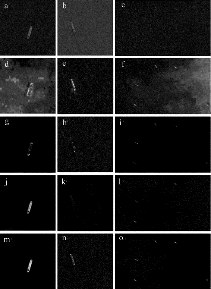
Figure 4. Different saliency map
a~c—original image d~f—Itti saliency map g~i—SR saliency map j~l—FT saliency map m~o—HC saliency map
![]()
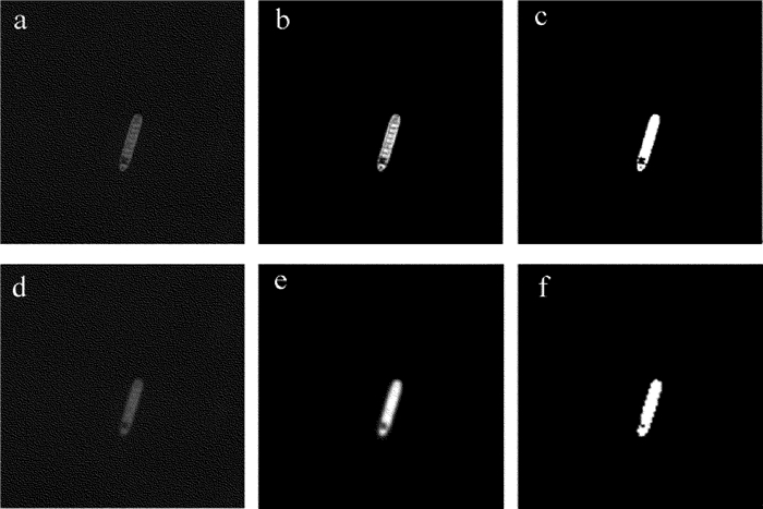
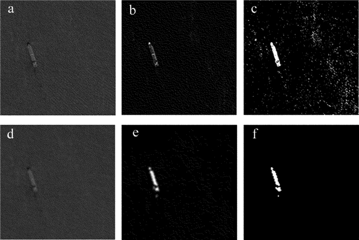
Figure 5. Comparison of ship detection results before and after dimension reduction of Fig. 4a
a—original image b—HC saliency map c—the result of segmentation d—the reduced dimension image e—HC saliency map after dimension reduction f—the result of segmentation after dimension reduction
![]()
Figure 6. Comparison of ship detection results before and after dimension reduction Fig. 4b
a—original image b—HC saliency map c—the result of segmentation d—the reduced dimension image e—HC saliency map after dimension reduction f—the result of segmentation after dimension reduction
![]()
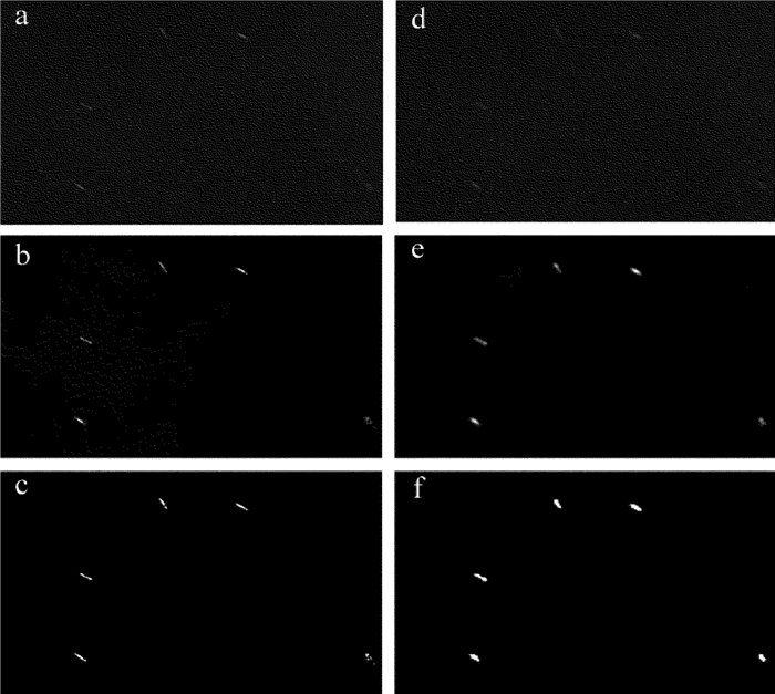
Figure 7. Comparison of ship detection results before and after dimension reduction of Fig. 4c
a—original image b—HC saliency map c—the result of segmentation d—the reduced dimension image e—HC saliency map after dimension reduction f—the result of segmentation after dimension reduction
Table 1 The processing time of different algorithms
the processing time/ms Itti SR FT H the first image
(512×512)2271.4 126.1 106.8 64.7 the second image
(512×512)2390.0 129.2 110.3 69.5 the third image
(1024×600)4895.2 286.9 235.7 106.1  下载: 导出CSV
Table 2 Comparison of target detection time
original image/ms Gaussian dimension reductionimage/ms the first image 73.4 8.9 the second image 78.4 9.1 the third image 121.9 12.6
下载: 导出CSV
-
[1] ZHANG Zh. A study on harbor target recognition in high resolution optical remote sensing image[D].Hefei: University of Science and Technology of China, 2005: 79-84(in Chinese).
[2] WANG M, LUO J Ch, MING D P. Extract ship targets from high spatial resolution remote sensed imagery with shape feature[J]. Geomatics and Information Science of Wuhan University, 2005, 30(8):685-688(in Chinese). http://www.wanfangdata.com.cn/details/detail.do?_type=perio&id=whchkjdxxb200508007
[3] CHU Zh L, WANG Q H, CHEN H L, et al. Ship auto detection method based on minimum error threshold segmentation[J]. Computer Engineering, 2007, 33(11):239-241(in Chinese). http://www.wanfangdata.com.cn/details/detail.do?_type=perio&id=jsjgc200711086
[4] XIAO L P, CAO J, GAO X Y. Detection for ship targets in complicated background of sea and land[J]. Opto-Electronic Engineering, 2007, 34(6):6-10(in Chinese). http://www.wanfangdata.com.cn/details/detail.do?_type=perio&id=gdgc200706002
[5] ZHAO Y H, WU X Q, WEN L Y, et al. Ship target detection scheme for optical remote sensing images[J]. Opto-Electronic Engineering, 2008, 35(8):102-106(in Chinese). http://cn.bing.com/academic/profile?id=dbaa175021e019edc35cfd41b95c9773&encoded=0&v=paper_preview&mkt=zh-cn
[6] XU J, XIANG J Y, ZHOU X, et al. A target segmentation algorithm based on feature field[J]. Infrared and Laser Engineering, 1998, 27(2):21-24(in Chinese). http://proceedings.spiedigitallibrary.org/mobile/proceeding.aspx?articleid=972077
[7] ZHU C, ZHOU H, WANG R, et al. A novel hierarchical method of ship detection from spaceborne optical image based on shape and texture features[J]. IEEE Transactions on Geoscience & Remote Sensing, 2010, 48(9):3446-3456. http://ieeexplore.ieee.org/document/5454348/
[8] WANG F Ch, ZHANG M, GONG L M, et al. Fast detection algorithm for ships under the background of ocean[J].Laser & Infrared, 2016, 46(5):602-606(in Chinese). http://www.wanfangdata.com.cn/details/detail.do?_type=perio&id=jgyhw201605019
[9] ZHANG L B, WANG P F. Fast detection of regions of interest in high resolution remote sensing image[J].Chinese Journal of Lasers, 2012, 39(7):714001(in Chinese). DOI: 10.3788/CJL
[10] ITTI L, KOCH C, NIEBUR E. A model of saliency-based visual attention for rapid scene analysis[J]. IEEE Transactions on Pattern Analysis & Machine Intelligence, 1998, 20(11):1254-1259. http://www.wanfangdata.com.cn/details/detail.do?_type=perio&id=ccf9901cbf11daa9b1aaa3928f527cbf
[11] HOU X, ZHANG L. Saliency detection: a spectral residual approach[C]//Computer Vision and Pattern Recognition CVPR 2007.New York, USA: IEEE, 2007: 1-8.
[12] ACHANTA R, HEMAMI S, ESTRADA F, et al. Frequency-tuned salient region detection[C]//Computer Vision and Pattern Recognition CVPR 2009.New York, USA: IEEE, 2009: 1597-1604.
[13] CHENG M M, ZHANG G X, MITRA N J, et al. Global contrast based salient region detection[C]//IEEE Conference on Computer Vision and Pattern Recognition. New York, USA: IEEE, 2011: 409-416.
[14] CHENG M M. Saliency and similarity detection for image scene analysis[D].Beijing: Tsinghua University, 2012: 31-53(in Chinese).
[15] WEI Y. Research on image salient region detection methods and applications[D].Ji'nan: Shandong University, 2012: 35-46(in Chinese).
[16] WANG Y W, LIANG Y Y, WANG Zh H. Otsu image threshold segmentation method based on new genetic algorithm[J]. Laser Technology, 2014, 38(3):364-367(in Chinese). http://d.old.wanfangdata.com.cn/Periodical/xtfzxb201706010
[17] WEI X F, LIU X. Research of image segmentation based on 2-D maximum entropy optimal threshold[J]. Laser Technology, 2013, 37(4):519-522(in Chinese). http://www.wanfangdata.com.cn/details/detail.do?_type=perio&id=jgjs201304023
[18] ZHANG J B, YANG H X, ZHOU T T, et al.Improved segmentation method of 2-D Otsu infrared image[J]. Laser Technology, 2014, 38(5):713-717(in Chinese). http://www.wanfangdata.com.cn/details/detail.do?_type=perio&id=jgjs201405029


计量
- 文章访问数: 7
- HTML全文浏览量: 0
- PDF下载量: 16