 网站地图
网站地图


-
结构光3维形貌测量技术是当今社会一种应用广泛的技术,因其具有非接触式、全场测量、低成本等优点, 在工业制造、物品3维轮廓检测、人体建模、航天领域和医学领域等众多领域具有庞大的技术需求[1]。其中条纹投影轮廓术是结构光3维形貌测量中最具有代表性的一项技术[2]。条纹投影轮廓术原理是先用投影仪将光栅条纹投射到被测物体表面,然后光栅变形条纹与参考条纹由摄像机捕获,被摄像机捕获到的条纹通过计算可以求出内含被测物体高度信息的包裹相位,然后通过相位展开求取真实相位,最后利用相位-高度映射和摄像机-投影仪条纹投影轮廓术(fringe projection profilometry,FPP)系统的标定参数,进行3维重建[3-4]、生成3维点云[5]。摄像机进行条纹捕获时会引入噪声[6], 从而造成相位误差,最终会影响3维重建的精确度。
对于条纹投影轮廓术,条纹噪声通常是不可避免的,并导致相位误差。目前,很多学者对噪声所致的相位误差和相位展开可靠性进行了研究。WANG等人[7]提出一种边缘模式策略,通过最大化计算长度来提高模式信噪比,但这种技术对投影仪与相机之间的图像散焦和分辨率差异很敏感。YANG[8]提出了基于2维正弦光栅编码的系统标定,消除了投影仪镜头畸变引起的测量误差。CUI等人[9]提出一种基于π/3相移的噪声补偿方法,通过相移则可以使信号的强度反转,噪声强度也反转,相移前后的噪声叠加取均值来补偿噪声。ZUO等人[10]利用捕获条纹的调制强度与相位误差成反比的特点,提出了一种提高获取条纹调制强度的方法。SERVIN等人[11]证实相移条纹噪声通常为高斯噪声,相位误差也符合高斯随机过程。LI等人[12]用随机噪声方差表达相位误差,使随机噪声方差与相位误差建立联系,证明相位误差与相移步数成反比、与捕获条纹的调制强度成反比、与随机噪声方差的平方成正比,并且得出相位方差与条纹频率有关,并给出条纹最优频率及其偏差所带来的误差。ZHUANG等人[13]通过处理采集条纹,提取被测物体的轮廓,精确定位噪声范围,并对误差像素均值化来减小噪声带来的误差。BAI[14]针对优化结构光条纹图像质量,通过滤波方法解决了结构光条纹图像灰度分布退化的问题。
条纹噪声是随机的,但现有方法的噪声模型是基于高斯噪声模型。此外,现有方法仅讨论标准的双频或多频相移法(如3fh+3fl、4fh+4fl,表示三步或四步相移双频外差方法, fh和fl分别表示高频和低频),尚未对非标准的双频或多频相移法(如3fh+2fl,表示高频三步相移和低频两步相移双频外差方法)进行讨论与分析。为此,本文作者提出了一种评价方法,该方法不基于高斯噪声模型,直接根据条纹噪声的方差计算相位误差的最大方差;然后讨论了3种双频相移法(标准3fh+3fl与4fh+4fl,非标准的3fh+2fl)相位展开的可靠性; 理论与实验对比了3种算法的包裹相位误差和相位展开可靠性。
-
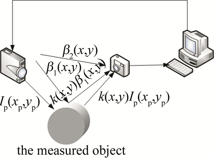
光栅投影原理是在被测物体的表面投影计算机生成的标准正弦光栅条纹,通常采用相移法[15],被测物体表面上的变形条纹由相机采集传输给计算机,最后通过相机采集到的参考条纹和被测物体表面的变形条纹计算出相位。假设光栅投影条纹为正弦条纹,则投影条纹的灰度值可以由下式表示[16]:
$ \begin{gather*} I_{\mathrm{p}}\left(x_{\mathrm{p}}, y_{\mathrm{p}}\right)=A\left(x_{\mathrm{p}}, y_{\mathrm{p}}\right)+ \\ B\left(x_{\mathrm{p}}, y_{\mathrm{p}}\right) \cos \left(2 {\rm{ \mathsf{ π} }} f_{0} x_{\mathrm{p}}\right) \end{gather*} $
(1) 式中: Ip(xp, yp)表示投影仪所投影的条纹; A(xp, yp)为背景光强值; B(xp, yp)为调制强度; f0为载波频率。投影相移条纹的灰度值可以用下式表示:
$ \begin{gather*} I_{n, \mathrm{p}}\left(x_{\mathrm{p}}, y_{\mathrm{p}}\right)=A\left(x_{\mathrm{p}}, y_{\mathrm{p}}\right)+ \\ B\left(x_{\mathrm{p}}, y_{\mathrm{p}}\right) \cos \left(2 {\rm{ \mathsf{ π} }} f_{0} x_{\mathrm{p}}+p_{n}\right) \end{gather*} $
(2) 式中: n表示第n次相移; pn=2π(n-1)/N; N表示相移步长总数。相机采集过程中会受到周围环境光和被测物体表面反光的干扰,因此摄像机采集到的光栅条纹表示为:
$ \begin{gather*} I_{n, \mathrm{c}}\left(x_{\mathrm{c}}, y_{\mathrm{c}}\right)=a\left(x_{\mathrm{c}}, y_{\mathrm{c}}\right)+ \\ b\left(x_{\mathrm{c}}, y_{\mathrm{c}}\right) \cos \left[\phi(x, y)+p_{n}\right] \end{gather*} $
(3) 式中:
$ \left\{\begin{align*} a\left(x_{\mathrm{c}}, y_{\mathrm{c}}\right)= & k(x, y)\left[A\left(x_{\mathrm{p}}, y_{\mathrm{p}}\right)+\right. \\ & \left.\beta_{1}(x, y)\right]+\beta_{2}(x, y) \\ b\left(x_{\mathrm{c}}, y_{\mathrm{c}}\right)= & k(x, y) B\left(x_{\mathrm{p}}, y_{\mathrm{p}}\right) \end{align*}\right. $
(4) 式中: In,c(xc,yc)表示摄像机所采集的条纹; ϕ(x, y)为包裹相位; k(x, y)为被测物体表面反射率; β1(x, y)为外部光源照到被测物体表面反射进入相机的环境光; β2(x, y)为外部光源直射相机的环境光。条纹投影与采集原理图如图 1所示。
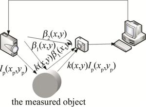
图 1 条纹投影与采集原理
Figure 1. Principle of fringe projection and capture
由相机捕获的条纹通过相位计算可以求出相位主值(也称为包裹相位),包裹相位求取由下式表示:
$ \begin{equation*} \phi(x, y)=-\arctan \left[\frac{\sum\limits_{n=1}^{N} I_{n}(x, y) \sin p_{n}}{\sum\limits_{n=1}^{N} I_{n}(x, y) \cos p_{n}}\right] \end{equation*} $
(5) 式中: ϕ(x, y)的范围限制在-π和π之间,为了建立相机和投影仪间唯一的像素对应关系,并正确重建3维形貌,需对相位进行展开[17],而展开相位的计算方法有空间相位展开法和时间相位展开法[18-20],本文中采用时间相位展开法求展开相位,这种方法对于复杂的物体形貌依然可以准确计算出展开相位,对于表面不连续的物体依然可以精确测量[21]。典型的时间相位展开法有三频相位展开法、三频外差相位展开法、指数增长、线性增长、负指数增长,本文作者采用双频外差法来求解包裹相位,然后通过解出频率为1的包裹相位间接求取展开相位。
-
通过摄像机捕获条纹频率为fh和fl的投影条纹灰度值可以表示为:
$ \left\{\begin{align*} I_{m, f_{\mathrm{h}}}(x, y)= & a\left(x_{\mathrm{c}}, y_{\mathrm{c}}\right)+b\left(x_{\mathrm{c}}, y_{\mathrm{c}}\right) \times \\ & \cos \left[2 {\rm{ \mathsf{ π} }} m / M+\phi_{f_{\mathrm{h}}}(x, y)\right] \\ I_{n, f_{\mathrm{l}}}(x, y)= & a\left(x_{\mathrm{c}}, y_{\mathrm{c}}\right)+b\left(x_{\mathrm{c}}, y_{\mathrm{c}}\right) \times \\ & \cos \left[2 {\rm{ \mathsf{ π} }} n / N+\phi_{f_{1}}(x, y)\right] \end{align*}\right. $
(6) 式中: fh表示高频; m(m=0, 1, 2,…, M-1)是指频率为fh的捕获光栅条纹的相移步数; M是指频率为fh的捕获光栅条纹的相移步长总数, 这里M=3;fl表示低频; n(n=0, 1, 2,…, N-1)是指频率为fl的捕获光栅条纹的相移步数; N是指频率为fl的捕获光栅条纹的相移步长总数,这里N=3。频率为fh的三步相移的包裹相位可以表示为:
$ \begin{gather*} \phi_{3 s, f_{\mathrm{h}}}(x, y)= \\ \arctan \left\{\frac{\sqrt{3}\left[I_{3, f_{\mathrm{h}}}(x, y)-I_{2, f_{\mathrm{h}}}(x, y)\right]}{2 I_{1, f_{\mathrm{h}}}(x, y)-I_{2, f_{\mathrm{h}}}(x, y)-I_{3, f_{\mathrm{h}}}(x, y)}\right\} \end{gather*} $
(7) 式中: ϕ3s,fh(x, y)表示高频三步相移; In, fh(x, y)(n=1, 2, 3)表示三步相移的第1幅、第2幅和第3幅条纹。
噪声干扰光栅条纹可以表示为:
$ \begin{equation*} G_{m, f_{\mathrm{h}}}(x, y)=I_{m, f_{\mathrm{h}}}(x, y)+N_{m, f_{\mathrm{h}}}(x, y) \end{equation*} $
(8) 式中: Nm, fh(x, y)是指在光栅条纹频率为fh的第m(m=1, 2, 3)个条纹的噪声强度。同理,由通式可以推出带噪声的三步相移的实际包裹相位可以表示为:
$\begin{array}{c} Q_{3 s, f_{\mathrm{h}}}(x, y)=\\ \arctan \left\{\frac{\sqrt{3}\left[G_{3, f_{\mathrm{h}}}(x, y)-G_{2, f_{\mathrm{h}}}(x, y)\right]}{2 G_{1, f_{\mathrm{h}}}(x, y)-G_{2, f_{\mathrm{h}}}(x, y)-G_{3, f_{\mathrm{h}}}(x, y)}\right\}= \\ \arctan \left\{\left[\sqrt{3}\left[I_{3, f_{\mathrm{h}}}(x, y)-I_{2, f_{\mathrm{h}}}(x, y)\right]+\nabla N_{1}(x, y)\right] \div\right.\\ \left.\left[2 I_{1, f_{\mathrm{h}}}(x, y)-I_{2, f_{\mathrm{h}}}(x, y)-I_{3, f_{\mathrm{h}}}(x, y)+\nabla N_{2}(x, y)\right]\right\} \end{array} $
(9) $ \left\{ \begin{array}{l} \nabla {N_1}(x,y) = \sqrt 3 \left[ {{N_{3,{f_{\rm{h}}}}}(x,y) - {N_{2,{f_{\rm{h}}}}}(x,y)} \right]\\ \nabla {N_2}(x,y) = \left[ {{N_{1,{f_{\rm{h}}}}}(x,y) - {N_{2,{f_{\rm{h}}}}}(x,y)} \right] + \\ \;\;\;\;\;\;\;\;\;\;\;\;\;\;\;\;\;\;\left[ {{N_{1,{f_{\rm{h}}}}}(x,y) - {N_{3,{f_{\rm{h}}}}}(x,y)} \right] \end{array} \right. $
(10) 为了便于计算,将符号后的(x, y)进行省略,根据式(7)、式(9)和式(10),噪声干扰引起的包裹相位误差可以表示为:
$ \begin{array}{c} \nabla \phi_{3 \mathrm{~s}, f_{\mathrm{h}}}=Q_{3 \mathrm{~s}, f_{\mathrm{h}}}-\phi_{3 \mathrm{~s}, f_{\mathrm{h}}}=\arctan \left[\tan \left(Q_{3 \mathrm{~s}, f_{\mathrm{h}}}-\phi_{3 \mathrm{~s}, f_{\mathrm{h}}}\right)\right]=\\ \arctan \left(\frac{\tan Q_{3 \mathrm{~s}, f_{\mathrm{h}}}-\tan \phi_{3 \mathrm{~s}, f_{\mathrm{h}}}}{1+\tan Q_{3 \mathrm{~s}, f_{\mathrm{h}}} \tan \phi_{3 \mathrm{~s}, f_{\mathrm{h}}}}\right)= \\ \arctan \left\{\left[\left(\sqrt{3}\left(I_{3, f_{\mathrm{h}}}-I_{2, f_{\mathrm{h}}}\right)+\nabla N_{1}\right)\left(2 I_{1, f_{\mathrm{h}}}-I_{2, f_{\mathrm{h}}}-I_{3, f_{\mathrm{h}}}\right)-\right.\right.\\ \left.\left(2 I_{1, f_{\mathrm{h}}}-I_{2, f_{\mathrm{h}}}-I_{3, f_{\mathrm{h}}}+\nabla N_{2}\right)\left(\sqrt{3}\left(I_{3, f_{\mathrm{h}}}-I_{2, f_{\mathrm{h}}}\right)\right)\right] \div \\ \left[\left(2 I_{1, f_{\mathrm{h}}}-I_{2, f_{\mathrm{h}}}-I_{3, f_{\mathrm{h}}}+\nabla N_{2}\right)\left(2 I_{1, f_{\mathrm{h}}}-I_{2, f_{\mathrm{h}}}-I_{3, f_{\mathrm{h}}}\right)+\right.\\ \left.\left.\left(\sqrt{3}\left(I_{3, f_{\mathrm{h}}}-I_{2, f_{\mathrm{h}}}\right)+\nabla N_{1}\right)\left(\sqrt{3}\left(I_{3, f_{\mathrm{h}}}-I_{2, f_{\mathrm{h}}}\right)\right)\right]\right\} \end{array} $
(11) 根据式(6)、式(8)和式(11),包裹相位误差可以进一步表示为:
$ \begin{align*} & \nabla \phi_{3 s, f_{\mathrm{h}}}=\\ &\arctan \left[\frac{\left(3 b\left(x_{\mathrm{c}}, y_{\mathrm{c}}\right) \sin \phi_{3 \mathrm{~s}, f_{\mathrm{h}}}+\nabla N_{1}\right) 3 b\left(x_{\mathrm{c}}, y_{\mathrm{c}}\right) \cos \phi_{3 \mathrm{~s}, f_{\mathrm{h}}}-\left(3 b\left(x_{\mathrm{c}}, y_{\mathrm{c}}\right) \cos \phi_{3 \mathrm{~s}, f_{\mathrm{h}}}+\nabla N_{2}\right) 3 b\left(x_{\mathrm{c}}, y_{\mathrm{c}}\right) \sin \phi_{3 \mathrm{~s}, f_{\mathrm{h}}}}{\left(3 b\left(x_{\mathrm{c}}, y_{\mathrm{c}}\right) \cos \phi_{3 \mathrm{~s}, f_{\mathrm{h}}}+\nabla N_{2}\right) 3 b\left(x_{\mathrm{c}}, y_{\mathrm{c}}\right) \cos \phi_{3 \mathrm{~s}, f_{\mathrm{h}}}+\left(3 b\left(x_{\mathrm{c}}, y_{\mathrm{c}}\right) \sin \phi_{3 \mathrm{~s}, f_{\mathrm{h}}}+\nabla N_{1}\right) 3 b\left(x_{\mathrm{c}}, y_{\mathrm{c}}\right) \sin \phi_{3 \mathrm{~s}, f_{\mathrm{h}}}}\right]= \\ & \arctan \left[\frac{3 b\left(x_{\mathrm{c}}, y_{\mathrm{c}}\right) \nabla N_{1} \cos \phi_{3 \mathrm{~s}, f_{\mathrm{h}}}-3 b\left(x_{\mathrm{c}}, y_{\mathrm{c}}\right) \nabla N_{2} \sin \phi_{3 \mathrm{~s}, f_{\mathrm{h}}}}{9 b\left(x_{\mathrm{c}}, y_{\mathrm{c}}\right)^{2}+3 b\left(x_{\mathrm{c}}, y_{\mathrm{c}}\right) \nabla N_{1} \sin \phi_{3 \mathrm{~s}, f_{\mathrm{h}}}+3 b\left(x_{\mathrm{c}}, y_{\mathrm{c}}\right) \nabla N_{2} \cos \phi_{3 \mathrm{~s}, f_{\mathrm{h}}}}\right]=\\ &\arctan \left(\frac{\nabla N_{1} \cos \phi_{3 s}-\nabla f_{\mathrm{h}}-\nabla N_{2} \sin \phi_{3 \mathrm{~s}, f_{\mathrm{h}}}}{3 b+\nabla N_{1} \sin \phi_{3 \mathrm{~s}, f_{\mathrm{h}}}+\nabla N_{2} \cos \phi_{3 \mathrm{~s}, f_{\mathrm{h}}}}\right) \end{align*} $
(12) 噪声强度远小于调制强度3b,因此上式可以简化为:
$ \begin{equation*} \nabla \phi_{3 \mathrm{~s}, f_{\mathrm{h}}}=\arctan \left[\frac{\nabla N_{1} \cos \phi_{3 \mathrm{~s}, f_{\mathrm{h}}}-\nabla N_{2} \sin \phi_{3 \mathrm{~s}, f_{\mathrm{h}}}}{3 b\left(x_{\mathrm{c}}, y_{\mathrm{c}}\right)}\right] \end{equation*} $
(13) 含有噪声的条纹计算的包裹相位减去理想条纹计算的包裹相位,并按如下方式计算方差:
$ \left\{\begin{array}{l} \operatorname{var}\left(N_{1}-N_{2}\right)=\operatorname{var}\left(N_{1}\right)+\operatorname{var}\left(N_{2}\right)-2 C\left(N_{1}, N_{2}\right) \\ \operatorname{var}\left(N_{1}-N_{3}\right)=\operatorname{var}\left(N_{1}\right)+\operatorname{var}\left(N_{3}\right)-2 C\left(N_{1}, N_{3}\right) \\ \operatorname{var}\left(N_{3}-N_{2}\right)=\operatorname{var}\left(N_{3}\right)+\operatorname{var}\left(N_{2}\right)-2 C\left(N_{3}, N_{2}\right) \end{array}\right. $
(14) 式中,var(·)代表求方差,C(·)表示相关系数。
由于三步相移条纹由相同的测量系统捕获,因此可以假设随机噪声方差大致相等,式(10)可以进一步表示为:
$ \left\{\begin{align*} \nabla N_{1}(x, y)= & \sqrt{3}\left[N_{3, f_{\mathrm{h}}}(x, y)-N_{2, f_{\mathrm{h}}}(x, y)\right] \Rightarrow \\ & \sigma_{\nabla 1}^{2}=2 \sqrt{3} \sigma^{2}\left(1-\zeta_{3-2}\right)=2 \sqrt{3} \tau_{3-2} \sigma^{2} \\ \nabla N_{2}(x, y)= & {\left[N_{1, f_{\mathrm{h}}}(x, y)-N_{2, f_{\mathrm{h}}}(x, y)\right]+} \\ & {\left[N_{1, f_{\mathrm{h}}}(x, y)-N_{3, f_{\mathrm{h}}}(x, y)\right] \Rightarrow } \\ & \sigma_{\nabla 2}^{2}=2 \sigma^{2}\left(1-\zeta_{1-2}\right)+2 \sigma^{2}\left(1-\zeta_{1-3}\right)= \\ & 2 \tau_{1-2} \sigma^{2}+2 \tau_{1-3} \sigma^{2} \end{align*}\right. $
(15) 式中: σ2是噪声的方差; σ∇12是随机噪声差∇N1(x, y)的方差; σ∇22是随机噪声差∇N2(x, y)的方差; ζ是相关系数; ζ3-2表示第3幅与第2幅条纹的相关系数,并且0≤ζ≤1,τ=1-ζ,则0≤τ≤1。
为了容易比较相位误差,假设两个随机噪声的相关系数相等,则τ1-2=τ1-3=τ3-2=τ1,则可以推出:
$ \left\{\begin{array}{l} \sigma_{\nabla 1}^{2}=2 \sqrt{3} \tau_{1} \sigma^{2} \\ \sigma_{\nabla 2}^{2}=4 \tau_{1} \sigma^{2} \end{array}\right. $
(16) 因为∇N1(x, y)和∇N2(x, y)比b(xc, yc)小很多,而且使用相位误差的方差来表示它们的值,因此可以得出:
$ \begin{align*} \nabla \phi_{3 s, f_{\mathrm{h}}} & \approx \frac{\nabla N_{1} \cos \phi_{3 \mathrm{~s}, f_{\mathrm{h}}}-\nabla N_{2} \sin \phi_{3 \mathrm{~s}, f_{\mathrm{h}}}}{3 b\left(x_{\mathrm{c}}, y_{\mathrm{c}}\right)} \Rightarrow \\ \sigma_{\nabla \phi_{3 s}, f_{\mathrm{h}}}= & \frac{2 \sqrt{3} \tau_{1} \sigma^{2} \cos \phi_{3 \mathrm{~s}, f_{\mathrm{h}}}-4 \tau_{1} \sigma^{2} \sin \phi_{3 s, f_{\mathrm{h}}}}{3 b\left(x_{\mathrm{c}}, y_{\mathrm{c}}\right)} \end{align*} $
(17) 根据上式可以得出与之对应的方程式:
$ \begin{equation*} y=\sqrt{3} \cos \phi_{3 \mathrm{~s}, f_{\mathrm{h}}}-2 \sin \phi_{3 \mathrm{~s}, f_{\mathrm{h}}} \end{equation*} $
(18) 然后对上式ϕ3s, fh求导,可以求出y的极值。
令:
$ \begin{equation*} \frac{\mathrm{d} y}{\mathrm{~d} \phi_{3 \mathrm{~s}, f_{\mathrm{h}}}}=-\sqrt{3} \sin \phi_{3 \mathrm{~s}, f_{\mathrm{h}}}-2 \cos \phi_{3 \mathrm{~s}, f_{\mathrm{h}}}=0 \end{equation*} $
(19) 并且已知:
$ \begin{equation*} \sin ^{2} \phi_{3 s, f_{\mathrm{h}}}+\cos ^{2} \phi_{3 s, f_{\mathrm{h}}}=1 \end{equation*} $
(20) 因此频率为fh的三步相移的包裹相位误差的最大方差可以得出:
$ \begin{gather*} \left\{\begin{array}{l} \sin \phi_{3 \mathrm{~s}, f_{\mathrm{h}}}= \pm \frac{2}{\sqrt{7}} \\ \cos \phi_{3 \mathrm{~s}, f_{\mathrm{h}}}=\mp \frac{\sqrt{3}}{\sqrt{7}} \end{array} \Rightarrow\right. \\ \left|\max \sigma_{\nabla \phi_{3 s, J_{\mathrm{h}}}}^{2}\right|=\frac{2 \sqrt{7} \tau_{1} \sigma^{2}}{3 b\left(x_{\mathrm{c}}, y_{\mathrm{c}}\right)} \approx 1.7638 \frac{\tau_{1} \sigma^{2}}{b\left(x_{\mathrm{c}}, y_{\mathrm{c}}\right)} \end{gather*} $
(21) 用相同的方法可以求出频率fl的三步相移的包裹相位误差的最大方差:
$ \begin{equation*} \left|\max \sigma_{\nabla \phi_{3 s}, f_{\mathrm{h}}}^{2}\right| \approx 1.7638 \frac{\tau_{1} \sigma^{2}}{b\left(x_{\mathrm{c}}, y_{\mathrm{c}}\right)} \end{equation*} $
(22) 对于双频外差相位展开算法,可以从频率为fh和fl的包裹相位中提取频率f1=1的包裹相位。
$ \begin{gather*} \nabla \phi_{f_{1}}=\nabla \varphi_{f_{1}}=Q_{f_{1}}-\phi_{f_{1}}= \\ {\left[Q_{3 \mathrm{~s}, f_{\mathrm{h}}}-Q_{3 \mathrm{~s}, f_{1}}\right]-\left[\phi_{3 \mathrm{~s}, f_{\mathrm{h}}}-\phi_{3 \mathrm{~s}, f_{1}}\right]=} \\ {\left[Q_{3 \mathrm{~s}, f_{\mathrm{h}}}-\phi_{3 \mathrm{~s}, f_{\mathrm{h}}}\right]-\left[Q_{3 \mathrm{~s}, f_{1}}-\phi_{3 \mathrm{~s}, f_{1}}\right]=} \\ \nabla \phi_{3 \mathrm{~s}, f_{\mathrm{h}}}-\nabla \phi_{3 \mathrm{~s}, f_{1}} \end{gather*} $
(23) 式中:∇φfl是频率为fl条纹展开相位的误差。频率为1的3fh+3fl包裹相位误差的最大方差:
$ \begin{gather*} \left|\max \sigma_{\nabla \phi_{f_{1}}}{ }^{2}\right| \approx 3.5276 \frac{\tau_{2} \tau_{1} \sigma^{2}}{b\left(x_{\mathrm{c}}, y_{\mathrm{c}}\right)}, \\ \left(0 \leqslant \tau_{2} \leqslant 1\right) \end{gather*} $
(24) 具有高频fh的展开相位可以由下式求出:
$ \varphi_{f_{\mathrm{h}}}=\phi_{f_{\mathrm{h}}}+2 {\rm{ \mathsf{ π} }} k $
(25) $ k=r\left(\frac{T_{\mathrm{h}} \varphi_{f_{1}}-\phi_{f_{\mathrm{h}}}}{2 {\rm{ \mathsf{ π} }}}\right) $
(26) 式中: r(·)为舍入函数; k是整数条纹顺序; Th为展开条纹周期数。式(26)的分子中包含相位误差,为保证k的正确性,其分子的相位误差应满足以下条件:
$ \begin{equation*} -{\rm{ \mathsf{ π} }}<\left(T_{\mathrm{h}} \nabla \varphi_{f_{1}}-\nabla \phi_{f_{\mathrm{h}}}\right)<{\rm{ \mathsf{ π} }} \end{equation*} $
(27) 可以得出上式分子的相位误差的最大方差为:
$ \begin{gather*} \max \left(T_{\mathrm{h}} \nabla \varphi_{f_{1}}-\nabla \phi_{f_{\mathrm{h}}}\right) \approx \\ 3.5276 T_{\mathrm{h}} \frac{\tau_{2} \tau_{1} \sigma^{2}}{b\left(x_{\mathrm{c}}, y_{\mathrm{c}}\right)} \end{gather*} $
(28) 根据式(28)可以看出,Th越小,k的可靠性越高。然而当Th越小,展开相位的分辨率越低,为了提高相位精度和k的可靠性,可以使用三频相移或多频相移。使用1.7638作为3fh+3fl的包裹相位误差系数,并且将3.5276作为3fh+3fl的展开相位可靠性。对于包裹相位可靠区域,包裹相位误差系数可用于表示最终相位精度,但是对于展开相位不可靠区域,由于条纹顺序引起的相位误差远大于包裹相位误差,因此使用相位展开可靠性系数来表示最终相位精度。
-
对于3fh+2fl,频率为fl的捕获条纹可以表示为:
$ \left\{\begin{align*} I_{1, f_{1}}= & a\left(x_{\mathrm{c}}, y_{\mathrm{c}}\right)+b\left(x_{\mathrm{c}}, y_{\mathrm{c}}\right) \cos \phi_{f_{1}} \\ I_{2, f_{1}}= & a\left(x_{\mathrm{c}}, y_{\mathrm{c}}\right)+b\left(x_{\mathrm{c}}, y_{\mathrm{c}}\right) \cos \left(\phi_{f_{1}}+{\rm{ \mathsf{ π} }} / 2\right)= \\ & a\left(x_{\mathrm{c}}, y_{\mathrm{c}}\right)-b\left(x_{\mathrm{c}}, y_{\mathrm{c}}\right) \sin \phi_{f_{1}} \end{align*}\right. $
(29) 频率为fl的二步相移计算包裹相位的方法为:
$ a\left(x_{\mathrm{c}}, y_{\mathrm{c}}\right)=\frac{I_{1, f_{\mathrm{h}}}+I_{2, f_{\mathrm{h}}}+I_{3, f_{\mathrm{h}}}}{3} $
(30) $ \begin{aligned} & \phi_{3 \mathrm{~s}, f_1}=\arctan \left[\frac{a\left(x_{\mathrm{c}}, y_{\mathrm{c}}\right)-I_{2, f_1}}{I_{1, f_l}-a\left(x_{\mathrm{c}}, y_{\mathrm{c}}\right)}\right]= \\ & \arctan \left(\frac{I_{1, f_{\mathrm{h}}}+I_{2, f_{\mathrm{h}}}+I_{3, f_{\mathrm{h}}}-3 I_{2, f_1}}{3 I_{1, f_1}-I_{1, f_{\mathrm{h}}}-I_{2, f_{\mathrm{h}}}-I_{3, f_{\mathrm{h}}}}\right) \end{aligned} $
(31) 对于3fh+2fl,频率为fh的最大包裹相位误差已经得到,频率为fl的最大包裹相位误差可由下式得出:
$ \begin{gathered} \nabla \phi_{2 \mathrm{~s}, f_{1}}=Q_{2 \mathrm{~s}, f_{1}}-\phi_{2 \mathrm{~s}, f_{1}}=\arctan \left[\tan \left(Q_{2 \mathrm{~s}, f_{1}}-\phi_{2 \mathrm{~s}, f_{1}}\right)\right]=\arctan \left(\frac{\tan Q_{2 \mathrm{~s}, f_{1}}-\tan \phi_{2 \mathrm{~s}, f_{1}}}{1+\tan Q_{2 \mathrm{~s}, f_{\mathrm{l}}} \tan \phi_{2 \mathrm{~s}, f_{1}}}\right)= \\ \arctan \left\{\left[\left(I_{1, f_{\mathrm{h}}}+I_{2, f_{\mathrm{h}}}+I_{3, f_{\mathrm{h}}}-3 I_{2, f_{\mathrm{h}}}+\nabla N_{1}\right)\left(3 I_{1, f_{\mathrm{h}}}-I_{1, f_{\mathrm{h}}}-I_{2, f_{\mathrm{h}}}-I_{3, f_{\mathrm{h}}}\right)-\right.\right. \\ \left.\left(3 I_{1, f_{1}}-I_{1, f_{\mathrm{h}}}-I_{2, f_{\mathrm{h}}}-I_{3, f_{\mathrm{h}}}+\nabla N_{2}\right)\left(I_{1, f_{\mathrm{h}}}+I_{2, f_{\mathrm{h}}}+I_{3, f_{\mathrm{h}}}-3 I_{2, f_{1}}\right)\right] \div \\ {\left[\left(3 I_{1, f_{1}}-I_{1, f_{\mathrm{h}}}-I_{2, f_{\mathrm{h}}}-I_{3, f_{\mathrm{h}}}+\nabla N_{2}\right)\left(3 I_{1, f_{1}}-I_{1, f_{\mathrm{h}}}-I_{2, f_{\mathrm{h}}}-I_{3, f_{\mathrm{h}}}\right)+\right.} \\ \left.\left.\left(I_{1, f_{\mathrm{h}}}+I_{2, f_{\mathrm{h}}}+I_{3, f_{\mathrm{h}}}-3 I_{2, f_{1}}+\nabla N_{1}\right)\left(I_{1, f_{\mathrm{h}}}+I_{2, f_{\mathrm{h}}}+I_{3, f_{\mathrm{h}}}-3 I_{2, f_{1}}\right)\right]\right\}= \\ \arctan \left\{\frac{\left[3 b\left(x_{\mathrm{c}}, y_{\mathrm{c}}\right) \sin \phi_{2 \mathrm{~s}, f_{1}}+\nabla N_{1}\right]\left[3 b\left(x_{\mathrm{c}}, y_{\mathrm{c}}\right) \cos \phi_{2 \mathrm{~s}, f_{1}}\right]-\left[3 b\left(x_{\mathrm{c}}, y_{\mathrm{c}}\right) \cos \phi_{2 \mathrm{~s}, f_{1}}+\nabla N_{2}\right]\left[3 b\left(x_{\mathrm{c}}, y_{\mathrm{c}}\right) \sin \phi_{2 \mathrm{~s}, f_{l}}\right]}{\left[3 b\left(x_{\mathrm{c}}, y_{\mathrm{c}}\right) \cos \phi_{2 \mathrm{~s}, f_{1}}+\nabla N_{2}\right]\left[3 b\left(x_{\mathrm{c}}, y_{\mathrm{c}}\right) \cos \phi_{2 \mathrm{~s}, f_{1}}\right]+\left[3 b\left(x_{\mathrm{c}}, y_{\mathrm{c}}\right) \sin \phi_{2 \mathrm{~s}, f_{1}}+\nabla N_{1}\right]\left[3 b\left(x_{\mathrm{c}}, y_{\mathrm{c}}\right) \sin \phi_{2 \mathrm{~s}, f_{1}}\right]}\right\} \approx\\ \frac{\nabla N_{1} \cos \phi_{2 \mathrm{~s}, f_{1}}-\nabla N_{2} \sin \phi_{2 \mathrm{~s}, f_{1}}}{3 b\left(x_{\mathrm{c}}, y_{\mathrm{c}}\right)} \end{gathered} $
(32) 式中: ϕ2s, fl表示低频两步相移。
为了比较相位误差,假设两个随机噪声的相关系数相等。
$ \left\{\begin{align*} \nabla N_{1}= & \left(N_{1, f_{\mathrm{h}}}-N_{2, f_{1}}\right)+\left(N_{2, f_{\mathrm{h}}}-N_{2, f_{1}}\right)+ \\ & \left(N_{3, f_{\mathrm{h}}}-N_{2, f_{1}}\right) \Rightarrow \sigma_{\nabla 1}^{2}=6 \tau_{1} \sigma^{2} \\ \nabla N_{2}= & \left(N_{1, f_{1}}-N_{1, f_{\mathrm{h}}}\right)+\left(N_{1, f_{1}}-N_{2, f_{\mathrm{h}}}\right)+ \\ & \left(N_{1, f_{1}}-N_{3, f_{\mathrm{h}}}\right) \Rightarrow \sigma_{\nabla 2}^{2}=6 \tau_{1} \sigma^{2} \end{align*}\right. $
(33) 则频率为fl的最大包裹相位为:
$ \begin{equation*} \left|\max \sigma_{\nabla \phi_{2 s, f_{1}}}^{2}\right| \approx 2.828 \frac{\tau_{1} \sigma^{2}}{b\left(x_{\mathrm{c}}, y_{\mathrm{c}}\right)} \end{equation*} $
(34) 讨论一下包裹相位的可靠性系数,通过3fh+2fl可以得到频率为1的包裹相位误差的最大方差:
$ |\max {\sigma _{\nabla {\phi _{{f_1}}}}}^2| \approx 4.5918\frac{{{\tau _2}{\tau _1}{\sigma ^2}}}{{b\left( {{x_c}, {y_c}} \right)}} $
(35) 3fh+2fl的展开相位的可靠性为:
$ \begin{equation*} \max \left(T_{\mathrm{h}} \nabla \varphi_{f_{1}}-\nabla \phi_{f_{\mathrm{h}}}\right) \approx 4.5918 T_{\mathrm{h}} \frac{\tau_{2} \tau_{1} \sigma^{2}}{b\left(x_{\mathrm{c}}, y_{\mathrm{c}}\right)} \end{equation*} $
(36) 对于展开相位可靠区域,包裹相位误差系数1.7638可用于表示最终相位精度。但是,对于相位展开不可靠区域,必须使用相位展开可靠性系数4.5918来表示最终相位精度。
-
频率为fh的四步相移包裹相位可以表示为:
$ \begin{equation*} \phi_{4 \mathrm{~s}, f_{\mathrm{h}}}=\arctan \left(\frac{I_{4, f_{\mathrm{h}}}-I_{2, f_{\mathrm{h}}}}{I_{1, f_{\mathrm{h}}}-I_{3, f_{\mathrm{h}}}}\right) \end{equation*} $
(37) 带噪声的四步相移的实际包裹相位可以表示为:
$ \begin{equation*} Q_{4 \mathrm{~s}, f_{\mathrm{h}}}=\arctan \left(\frac{I_{4, f_{\mathrm{h}}}-I_{2, f_{\mathrm{h}}}+\nabla N_{1}}{I_{1, f_{\mathrm{h}}}-I_{3, f_{\mathrm{h}}}+\nabla N_{2}}\right) \end{equation*} $
(38) 噪声干扰引起的包裹相位误差表示为:
$ \begin{array}{c} \nabla \phi_{4 \mathrm{~s}, f_{\mathrm{h}}}=\arctan \left(\frac{\nabla N_{1} \cos \phi_{4 \mathrm{~s}, f_{\mathrm{h}}}-\nabla N_{2} \sin \phi_{4 \mathrm{~s}, f_{\mathrm{h}}}}{2 b+\nabla N_{1} \sin \phi_{4 \mathrm{~s}, f_{\mathrm{h}}}+\nabla N_{2} \cos \phi_{4 \mathrm{~s}, f_{\mathrm{h}}}}\right) \approx\\ \frac{\nabla N_{1} \cos \phi_{4 \mathrm{~s}, f_{\mathrm{h}}}-\nabla N_{2} \sin \phi_{4 \mathrm{~s}, f_{\mathrm{h}}}}{2 b\left(x_{\mathrm{c}}, y_{\mathrm{c}}\right)} \end{array} $
(39) 为了比较相位误差,假设两个随机噪声的相关系数相等。
$ \left\{\begin{array}{l} \nabla N_{1}=N_{4, f_{\mathrm{h}}}-N_{2, f_{\mathrm{h}}} \Rightarrow \sigma_{\nabla 1}^{2}=2 \tau_{1} \sigma^{2} \\ \nabla N_{2}=N_{1, f_{\mathrm{h}}}-N_{3, f_{\mathrm{h}}} \Rightarrow \sigma_{\nabla 2}^{2}=2 \tau_{1} \sigma^{2} \end{array}\right. $
(40) 使用相位误差的方差来表示其值,式(39)可以进一步表示为:
$ \begin{align*} \nabla \phi_{4 \mathrm{~s}, f_{\mathrm{h}}} & \approx \frac{\nabla N_{1} \cos \phi_{4 \mathrm{~s}, f_{\mathrm{h}}}-\nabla N_{2} \sin \phi_{4 \mathrm{~s}, f_{\mathrm{h}}}}{2 b\left(x_{\mathrm{c}}, y_{\mathrm{c}}\right)} \Rightarrow \\ \sigma_{\nabla \phi_{f_{\mathrm{h}}}}{ }^{2} & =\frac{2 \tau_{1} \sigma^{2} \cos \phi_{4 \mathrm{~s}, f_{\mathrm{h}}}-2 \tau_{1} \sigma^{2} \sin \phi_{4 \mathrm{~s}, f_{\mathrm{h}}}}{2 b\left(x_{\mathrm{c}}, y_{\mathrm{c}}\right)} \end{align*} $
(41) 频率为fh和fl的四步相移的包裹相位的最大方差为:
$ \begin{align*} & \left|\max \sigma_{\nabla \phi_{f_{\mathrm{h}}}}{ }^{2}\right|=\left|\max \sigma_{\nabla \phi_{f_{1}}}{ }^{2}\right|= \\ & \sqrt{2} \frac{\tau_{1} \sigma^{2}}{b\left(x_{\mathrm{c}}, y_{\mathrm{c}}\right)} \approx 1.414 \frac{\tau_{1} \sigma^{2}}{b\left(x_{\mathrm{c}}, y_{\mathrm{c}}\right)} \end{align*} $
(42) 频率为1时,4fh+4fl包裹相位误差的最大方差为:
$ \begin{equation*} \left|\max \sigma_{\nabla \phi_{f_{1}}}^{2}\right| \approx 2.828 \frac{\tau_{2} \tau_{1} \sigma^{2}}{b\left(x_{\mathrm{c}}, y_{\mathrm{c}}\right)} \end{equation*} $
(43) 4fh+4fl展开相位的可靠性为:
$ \begin{equation*} \max \left(T_{\mathrm{h}} \nabla \varphi_{f_{1}}-\nabla \phi_{f_{\mathrm{h}}}\right) \approx 2.828 T_{\mathrm{h}} \frac{\tau_{2} \tau_{1} \sigma^{2}}{b\left(x_{\mathrm{c}}, y_{\mathrm{c}}\right)} \end{equation*} $
(44) 对于相位展开的可靠区域,包裹相位误差系数1.414可用于表示最终相位精度。但是对于相位展开不可靠区域,必须使用相位展开可靠性系数2.828来表示最终相位精度。
-
对于3fh+3fl,3fh+2fl和4fh+4fl,最终相位误差系数如表 1所示。对于相位展开可靠的区域,4fh+4fl的相位误差最小。对于相位展开不可靠的区域,4fh+4fl的相位误差最小。
表 1 最终相位误差系数比较
Table 1. Coefficients comparison of final phase error
method wrapped phase error coefficient (reliable phase unwrapping area) phase unwrapping reliability coefficient (unreliable phase unwrapping area) 3fh+3fl 1.7638 3.5276 3fh+2fl 1.7638 4.5918 4fh+4fl 1.4140 2.8280 首先,由于不可避免的阴影和额外的噪声干扰,应使用相位展开可靠性系数作为最终相位误差系数。包裹相位误差系数仅用于部分可靠性区域。以4fh+4fl的2.828为分母,得到相位误差系数的比值,如表 1所示。对于双频外差相位展开法,fh≈fl,相位误差方差可以计算如下:
$ \left\{\begin{align*} \sigma_{4 f_{\mathrm{h}}+4 f_{\mathrm{l}}}^{2} \approx & f_{\mathrm{h}}^{2} \frac{2 \sigma^{2}}{4 b\left(x_{\mathrm{c}}, y_{\mathrm{c}}\right)^{2}}+f_{\mathrm{h}}^{2} \frac{2 \sigma^{2}}{4 b\left(x_{\mathrm{c}}, y_{\mathrm{c}}\right)^{2}}=f_{\mathrm{h}}^{2} \frac{\sigma^{2}}{b\left(x_{\mathrm{c}}, y_{\mathrm{c}}\right)^{2}} \\ \sigma_{3 f_{\mathrm{h}}+3 f_{\mathrm{l}}}^{2} \approx & f_{\mathrm{h}}^{2} \frac{2 \sigma^{2}}{3 b\left(x_{\mathrm{c}}, y_{\mathrm{c}}\right)^{2}}+f_{\mathrm{h}}^{2} \frac{2 \sigma^{2}}{3 b\left(x_{\mathrm{c}}, y_{\mathrm{c}}\right)^{2}} \approx \\ & 1.33 f_{\mathrm{h}}^{2} \frac{\sigma^{2}}{b\left(x_{\mathrm{c}}, y_{\mathrm{c}}\right)^{2}} \\ \sigma_{3 f_{\mathrm{h}}+2 f_{\mathrm{l}}}^{2} \approx & f_{\mathrm{h}}^{2} \frac{2 \sigma^{2}}{3 b\left(x_{\mathrm{c}}, y_{\mathrm{c}}\right)^{2}}+f_{\mathrm{h}}^{2} \frac{2 \sigma^{2}}{2 b\left(x_{\mathrm{c}}, y_{\mathrm{c}}\right)^{2}} \approx \\ & 1.67 f_{\mathrm{h}}^{2} \frac{\sigma^{2}}{b\left(x_{\mathrm{c}}, y_{\mathrm{c}}\right)^{2}} \end{align*}\right. $
(45) 使用式(45)中4fh+4fl的相位误差方差作为分母,得到相位误差方差的比值,如表 2所示。从表 2的比较可以证实本文中误差模型的正确性。
表 2 相位误差系数之比
Table 2. Coefficient ratio of phase error
ratio ratio of the phase error coefficient in Table 1 ratio of the phase error variance in equation (45) $ \frac{3 f_{\mathrm{h}}+3 f_1}{4 f_{\mathrm{h}}+4 f_1}$ 1.25 1.33 $ \frac{3 f_{\mathrm{h}}+2 f_1}{4 f_{\mathrm{h}}+4 f_1}$ 1.62 1.67 -
实验设备主要由数字投影仪(三星SP-P410M)、摄像机(大恒彩色相机DH-GV400UC)和计算机(AMD Ryzen 5 5600H with Radeon Graphics 3.30 GHz)组成。3维测量流程如图 2所示。
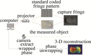
图 2 3维测量流程图
Figure 2. Flow chart of 3-D measurement
-
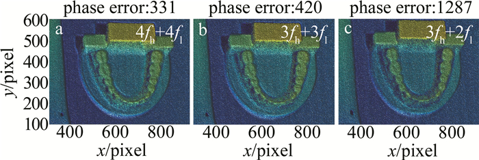
为了证明本文作者提出的评价方法,分别以小象和勺子工件为第1组实验对象,如图 3a所示;第2组实验对象为牙颌和牙膏,如图 4a所示。投影条纹周期数分别为33和32,通过以下3种方法3fh+2fl、3fh+3fl和4fh+4fl对物体进行相位计算和3维重建。图中的毛刺状相位误差由条纹噪声所致,其误差数量在图中用phase error(单位:个)表示。为了方便对比,给出了两个不同的视角,第一视角给出了物体重建形貌,第二视角便于观察噪声所致的噪声误差。第1组实验的重建正面效果如图 3b、图 3c和图 3d所示;其侧面效果如图 3e、图 3f和图 3g所示。第2组实验的重建正面效果如图 4b、图 4c、图 4d所示;其侧面效果如图 4e、图 4f和图 4g所示。
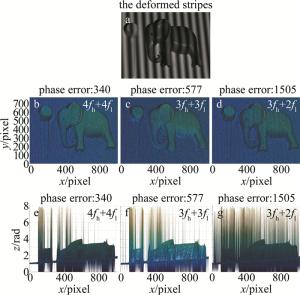
图 3 第1组实验的3维重建结果对比
Figure 3. Comparison of 3-D reconstruction results of the first group of experiments
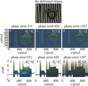
图 4 第2组实验的3维重建结果对比
Figure 4. Comparison of 3-D reconstruction results of the second group of experiments
表 3中为相位误差数量对比。可以看出,两组实验中4fh+4fl方法对物体进行3维重建后所产生的相位误差数量最少。相对于4fh+4fl方法,3fh+3fl方法提高了3维测量效率,但两种被测对象中,3fh+3fl方法的相位误差个数增加至4fh+4fl方法的169.7%和126.9%。3fh+2fl方法的条纹数量最少,测量效率最高,但3fh+2fl方法的相位误差个数增加至4fh+4fl方法的422.6%和388.8%。
表 3 相位误差数量对比
Table 3. Comparison of the number of phase errors
method the first group of experiments the second group of experiments 4fh+4fl 340 331 3fh+3fl 577 420 3fh+2fl 1505 1287 对图 4的重建正面效果图进行局部放大,结果如图 5所示。通过图 5中第2组实验的局部放大部分进行对比可以发现,用4fh+4fl方法对实验物体进行3维重建的效果要优于3fh+3fl和3fh+2fl,图 5a中重建平面比较光滑、完整,并且图像中出现的误差个数明显少于其它两个图像,而其它两种方法的实验结果中有比较严重的褶皱。比较3fh+2fl与3fh+3fl,对比图 5中的两种方法,由于3fh+2fl方法删减了部分条纹导致重建效果变差,相比3fh+3fl重建后的物体表面褶皱较明显,并且有些高光重建部分模糊,带有较多误差。因此,对比图 5b、图 5c可以发现,图 5c中重建表面褶皱较大并且不光滑,使用3fh+3fl方法对物体进行重建后的效果要优于3fh+2fl.,但相比于4fh+4fl算法和3fh+ 3fl算法,3fh+2fl方法测量效率提升了37.5%和16.6%。
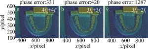
图 5 第2组实验的重建局部放大对比
Figure 5. Reconstruction of the second group of experiments with local amplification comparison
理论与实验结果表明,相位误差和相位展开可靠性与相移步数成反比,相移步数越高,则相位误差越小,相位展开可靠性越高,3维重建效果越好。但是,相移步数增大后,测量效率会降低。
-
在上述的两个实验中只是对物体表面进行局部放大对比,为了更精确地对3种方法进行比较,验证结论,将3种方法的3维重建结果取一行相位进行对比,对两组实验的结果都取第384行相位,以4fh+4fl方法进行重建的结果为例,对使用3种方法的结果提取第384行相位,其位置为图 6中红色虚线所标位置,红色方框中虚线为图 7中局部放大对比位置。
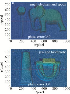
图 6 第384行相位及局部放大对比的位置
Figure 6. Position of phase and local amplification contrast in line 384
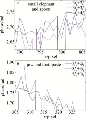
图 7 3种算法相位展开结果局部对比
Figure 7. Three algorithms phase unwrapping results are partial comparison
图 7中的洋红线、蓝线与黑线分别代表 3fh+2fl、3fh+3fl与4fh+4fl这3种方法的相位变化。从曲线可以看出,4fh+4fl所对应的黑线的波动要比其它两种颜色的线小很多,而3fh+3fl对应的蓝线与3fh+2fl对应的洋红线在4fh+4fl对应的黑线上下波动,但从整体看蓝线波动幅度略小于洋红线,3fh+3fl的相位波动略小于3fh+2fl的相位波动,并且洋红线垂直向下所代表的误差也要比其它两种方法多,因此验证了结论的准确性。
-
对于噪声引起的相位误差和相位展开的可靠性,本文中采取一种微分方法,引入方差,将随机噪声方差转化为相位误差的方差,通过微分来求取相位误差的最大方差,然后对比包裹相位误差系数和相位展开可靠性系数来判定3维重建效果的好坏。用第1、2组实验来对比3种方法3维重建后的效果,对结果进行局部放大对比分析与提取一行对比分析。对比结果验证了本方法的可靠性,实验验证了3种方法中4fh+4fl方法重建效果最佳,其重建物体表面平滑无褶皱,精度较高;其次是3fh+3fl算法的重建效果略差,重建物体表面散布水纹;最后是3fh+2fl算法重建模型褶痕较多,测量精度较差,但相比于传统算法将效率提升了37.5%。
噪声干扰的相位误差与相位展开可靠性研究
Research on phase error and phase unwrapping reliability of noise interference
-
摘要: 为了比较几种3维重建方法的优劣, 采用一种评价方法进行理论分析和实验验证, 建立了条纹噪声干扰的包裹相位误差模型, 求出包裹相位误差的最大方差, 然后对3种经典的双频相位展开算法的相位展开可靠性进行了分析和对比。结果表明, 双频四步相移算法4fh+4fl的抗干扰能力最强, 其重建物体表面平滑无褶皱; 其次是3fh+3fl算法, 其相位误差数量为4fh+4fl的169.7%和126.9%;3fh+2fl算法重建面形存在大量褶痕, 测量精度最差; 3fh+2fl算法的相位误差数量为4fh+4fl的442.6%和388.8%, 但相比于4fh+4fl算法和3fh+3fl算法, 测量效率提升了37.5%和16.6%。该研究为评价各双频相移法的优劣提供了一种方法, 并为以上3种算法的选择提供了参考。Abstract: In order to compare the advantages and disadvantages of several 3-D reconstruction methods, an evaluation method was adoped for theoretical analysis and experimental verification. The wrapped phase error model of fringe noise interference was established, and the maximum variance of the wrapped phase error was obtained. Then the reliability of three classical dual-frequency phase unwrapping algorithms was analyzed and compared. The results show that the dual-frequency four-step phase-shifting algorithm 4fh+4fl has the strongest anti-interference ability, and its reconstructed object surface is smooth and wrinkle-free. The second is the 3fh+3fl algorithm, whose phase errors are 169.7% and 126.9% of those of 4fh+4fl. Finally, the 3fh+2fl algorithm has a large number of folds on the reconstructed shapes, and the measurement accuracy is the worst. The phase errors of the 3fh+2fl algorithm are 442.6% and 388.8% of those of the 4fh+4fl algorithm. However, compared with the 4fh+4fl algorithm and the 3fh+3fl algorithm, the measurement efficiency is improved by 37.5% and 16.6%. This study provides a method to evaluate the advantages and disadvantages of each dual-frequency phase shift method and provides a reference for the selection of the above three methods.
-
Key words:
- gratings /
- noise /
- phase error /
- phase unwrapping reliability
-
图 3 第1组实验的3维重建结果对比
Figure 3. Comparison of 3-D reconstruction results of the first group of experiments
图 4 第2组实验的3维重建结果对比
Figure 4. Comparison of 3-D reconstruction results of the second group of experiments
图 5 第2组实验的重建局部放大对比
Figure 5. Reconstruction of the second group of experiments with local amplification comparison
图 6 第384行相位及局部放大对比的位置
Figure 6. Position of phase and local amplification contrast in line 384
图 7 3种算法相位展开结果局部对比
Figure 7. Three algorithms phase unwrapping results are partial comparison
表 1 最终相位误差系数比较
Table 1. Coefficients comparison of final phase error
method wrapped phase error coefficient (reliable phase unwrapping area) phase unwrapping reliability coefficient (unreliable phase unwrapping area) 3fh+3fl 1.7638 3.5276 3fh+2fl 1.7638 4.5918 4fh+4fl 1.4140 2.8280  下载: 导出CSV
表 2 相位误差系数之比
Table 2. Coefficient ratio of phase error
ratio ratio of the phase error coefficient in Table 1 ratio of the phase error variance in equation (45) $ \frac{3 f_{\mathrm{h}}+3 f_1}{4 f_{\mathrm{h}}+4 f_1}$ 1.25 1.33 $ \frac{3 f_{\mathrm{h}}+2 f_1}{4 f_{\mathrm{h}}+4 f_1}$ 1.62 1.67
下载: 导出CSV
表 3 相位误差数量对比
Table 3. Comparison of the number of phase errors
method the first group of experiments the second group of experiments 4fh+4fl 340 331 3fh+3fl 577 420 3fh+2fl 1505 1287
下载: 导出CSV
-
[1] 李中伟. 基于数字光栅投影的结构光三维测量技术与系统研究[D]. 武汉: 华中科技大学, 2009: 1-4. LI Zh W. Research on structural light 3D measurement technology and system based on digital fringe projec-tion[D]. Wuhan: Huazhong University of Science and Technology, 2009: 1-4(in Chinese). [2] 左超, 张晓磊, 胡岩, 等. 3D真的来了吗?——三维结构光传感器漫谈[J]. 红外与激光工程, 2020, 49(3): 0303001. ZUO Ch, ZHANG X L, HU Y, et al. Has 3D finally come of age?——An introduction to 3D structured-light sensor[J]. Infrared and Laser Enginering, 2020, 49(3): 0303001(in Chinese). [3] LI Y X, QIAN J M, FENG Sh J, et al. Deep learning-enabled dual-frequency composite fringe projection prof-ilometry for single-shot absolute 3D shape measurement[J]. Opto-Electronic Advances, 2022, 5(5): 210021. doi: 10.29026/oea.2022.210021 [4] FENG Sh J, ZUO Ch, ZHANG L, et al. Calibration of fringe projection profilometry: A comparative review[J]. Optics and Lasers in Engineering, 2021, 143: 106622. doi: 10.1016/j.optlaseng.2021.106622 [5] 巩育江, 庞亚军, 王汞, 等. 基于几何特征的点云分割算法研究进展[J]. 激光技术, 2022, 46(3): 326-336. GONG Y J, PANG Y J, WANG G, et al. Research progress of point clouds segmentation algorithms based on geometric features[J]. Laser Technology, 2022, 46(3): 326-336(in Chinese). [6] 陈念. 基于结构光视觉的植保无人机障碍物图像加速处理技术研究[D]. 杭州: 杭州电子科技大学, 2018: 18-36. CHEN N. Research on accelerated image processing technology of plant protection UAV based on structural light vision[D]. Hangzhou: Hangzhou Dianzi University, 2018: 18-36(in Chinese). [7] WANG Y Ch, LIU K, DANIEL L, et al. Maximum snr pattern strategy for phase shifting methods in structured light illumination[J]. Journal of the Optical Society of America, 2010, 27(9): 1962-1971. doi: 10.1364/JOSAA.27.001962 [8] 杨柳. 单目结构光三维测量精度优化技术研究[D]. 南京: 南京航空航天大学, 2017: 24-33. YANG L. Research on the precision optimization for the monocular structured light 3D measurement system[D]. Nanjing: Nanjing University of Aeronautics and Astronautics, 2017: 24-33(in Chinese). [9] 崔索超, 孙峰. 面结构光测量系统中基于π/3相移的噪声补偿算法[J]. 光学与光电技术, 2018, 16(4): 19-22. CUI S Ch, SUN F. Noise compensation algorithm based on π/3 phase shift in the surface structure light measurement system[J]. Optical and Optical Technology, 2018, 16(4): 19-22(in Chinese). [10] ZUO Ch, CHEN Q, GU G H, et al. Optimized three-step phase shifting profifilometry using the third harmonic injection[J]. Optica Applicata, 2013, 43(2): 393-408. [11] SERVIN M, ESTRADA J C, QUIROGA J A, et al. Noise in phase shifting interferometry[J]. Optics Express, 2009, 17(11): 8789-8794. doi: 10.1364/OE.17.008789 [12] LI J, HASSEBROOK LG, GUAN C. Optimized two-frequency phase measuring profi filometry light sensor temporal noise sensitivity[J]. Journal of the Optical Society of America, 2003, 20(1): 106-115. doi: 10.1364/JOSAA.20.000106 [13] 庄一, 石岩, 汪诗宇. 基于相移法的三维重建减噪算法研究[J]. 中国计量大学学报, 2018, 29(4): 446-451. ZHUANG Y, SHI Y, WANG Sh Y. Research on 3D reconstruction noise reduction algorithms based on the phase shifting method[J]. Journal of China University of Metrology, 2018, 29(4): 446-451(in Chinese). [14] 白杨. 结构光三维测量图像噪声分析与预处理方法研究[D]. 郑州: 郑州大学, 2019: 21-30. BAI Y. Study on noise analysis and preprocessing of structured light three-dimensional measurement image[D]. Zhengzhou: Zhengzhou University, 2019: 21-30(in Chinese). [15] ZUO Ch, FENG Sh J, HUANG L, et al. Phase shifting algorithms for fringe projection profilometry: A review[J]. Optics and Lasers in Engineering, 2018, 109: 23-59. doi: 10.1016/j.optlaseng.2018.04.019 [16] 王建华. 光栅投影三维测量关键技术研究[D]. 西安: 西安理工大学, 2019: 18-19. WANG J H. Research on key technologies of fringe projection 3D measurement[D]. Xi'an: Xi'an University of Technology, 2019: 18-19(in Chinese). [17] 左超, 陈钱. 计算光学成像: 何来, 何处, 何去, 何从?[J]. 红外与激光工程, 2022, 51(2): 20220110. ZUO Ch, CHEN Q. Computational optical imaging: An overview[J]. Infrared and Laser Engineering, 2022, 51(2): 20220110(in Chinese). [18] 张旭. 基于光栅投影的三维人脸识别研究与实现[D]. 石家庄: 河北科技大学, 2020: 25-26. ZHANG X. Research and implementation of 3-D face recognition based on raster projection[D]. Shijiazhang: Hebei University of Science and Technology, 2020: 25-26(in Chinese). [19] ZUO Ch, HUANG L, ZHANG M L, et al. Temporal phase unwrapping algorithms for fringe projection profilometry: A comparative review[J]. Optics and Lasers in Engineering, 2016, 85: 84-103. doi: 10.1016/j.optlaseng.2016.04.022 [20] ZHANG M, CHEN Q, TAO T, et al. Robust and efficient multi-frequency temporal phase unwrapping: Optimal fringe frequency and pattern sequence selection[J]. Optics Express, 2017, 25(17): 20381. doi: 10.1364/OE.25.020381 [21] 岳慧敏, 基于时间相位展开的三维轮廓测量研究[D]. 成都: 四川大学, 2005: 30-38. YUE H M. Research on three-dimensional profilometry based on temporal phase unwrapping[D]. Chengdu: Sichuan University, 2005: 30-38(in Chinese). -

 点击查看大图
计量
- 文章访问数: 1206
- HTML全文浏览量: 816
- PDF下载量: 11
- 被引次数: 0
