 网站地图
网站地图


-
激光加工技术[1]主要是利用激光束与物质相互作用的特性来对材料进行微加工。由于激光具有亮度高、方向性好、相干性好、单色性好等优点[2],使其在金属加工方面应用非常广泛。利用激光进行机械加工制造,不仅可以加工复杂形状,而且可以提高工作效率,具有非常广阔的应用场景。本文中使用激光完成一种过滤网的加工,首先需要在金属模具上加工一定数量不击穿的圆孔(定义此类圆孔为盲孔,定义盲孔的集合为网点),这些盲孔深度一定且规则分布,直径约为2mm~5mm,使用机械加工;然后在盲孔中使用激光加工一定数量的微孔[3],直径大小约为200μm,击穿金属模具。
过滤网的两步加工过程中,第1步网点的加工由于初始的金属模具未加工,根据网点理论图选定金属模具的某个位置作为起始点即可完成加工,定位简单;第2步在盲孔中加工微孔,和第1步相比,金属模具上已经有了很多规则分布、一定孔径的盲孔,且圆盘的位置已经改变,因此,若想在盲孔内部继续完成微孔的加工,就需要对网点进行精准定位,获知网点中盲孔在平台坐标系中的分布位置。原始的定位方法是使用人工定位,选中网点中的一些盲孔,使用激光尝试加工,依靠人眼判断打点是否准确,然后移动金属滤网直至激光打点基本准确,此种方法误差大、耗时长。另一种结合视觉定位的方法就是对整个网点拍照取像,将像素坐标转换成平台坐标,但是由于网点幅面较大,而相机的拍摄幅面较小,无法一次取像,只能通过图片拼接[4]的方法完成整个网点的采集,这极大地降低了工作效率。故本实验中采用局部定位整体的方法实现网点定位,获得盲孔在平台坐标系中的分布位置。该方法实现了平台的自动定位,不仅效率高,且定位准确。
-
本实验开发过程中使用的实验器材包含一个光纤激光器模组、2片x轴和y轴振镜、一块自主研发的振镜驱动卡、一个高精度工业相机、一个高精度移动平台。硬件平台搭建如图 1所示。
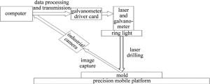
Figure 1. Experimental schematic
实验从建立振镜-相机-平台坐标系开始,建立统一的世界坐标系,方便坐标转换。采用的定位方案如图 2所示。
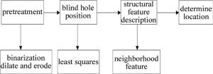
Figure 2. Scheme of point positioning
预处理中主要分为两部分:二值化[5]和膨胀腐蚀[6]。二值化的作用是消除图片中的噪声,膨胀可以使圆孔的轮廓更加清晰,腐蚀可以避免相邻的盲孔轮廓相连,根据实际情况选择其中一种。之后使用最小二乘法拟合得到盲孔的圆心坐标和半径,采用邻域特征法确定局部图像边缘点的特征描述,并和理论图像边缘点的特征描述进行对比,得到局部图像在理论图像的位置,计算偏移量和旋转角,实现金属滤网盲孔的定位,继续后续加工。
-
当前理论中,基于霍夫变换[7-9](Hough transform, HT)的圆识别是识别圆的经典算法之一。HT首先利用canny边缘检测算子检测边缘,并将边缘像素映射为3维的霍夫圆空间,然后提取包含一定像素的圆形[10]。该类方法不仅耗时、费空间,而且准确率低、很多参量需要用户给定。为了克服这些缺点,提出了很多改进算法,如随机霍夫变换[11]、模糊霍夫变换[12]、点霍夫变换[13]等。改进算法虽然某种程度上克服了经典HT的缺点,但速度仍然不能满足需要,而且准确率仍然不高。根据所研究的模型,本文中采用了提取圆轮廓点进行最小二乘法拟合圆[14-15]的识别方法。此种方法速度快、准确率高,而且圆心识别准确,能够满足需要。
-
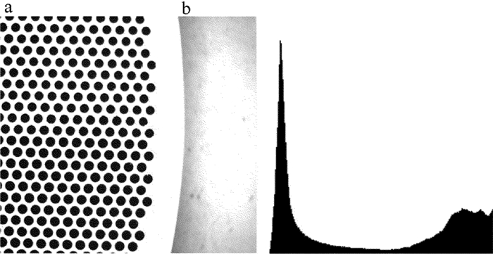
图像采集时需要对图像进行轻微的过曝处理,减少金属滤网表面纹理等造成的噪声,如图 3a所示。因为正常曝光的情况下,物体表面的纹理较为清晰,会影响图像二值化;过度曝光的情况下,盲孔的边缘会被过度腐蚀,直接干扰轮廓检测。

Figure 3. a—the captured image b—grayscale histogram
采集图像后,需要对图像进一步处理,去除多余噪声,保证盲孔轮廓的完整,提高识别轮廓的准确率。本文中采用的预处理方式有二值化、膨胀腐蚀等。根据相机采集图像的灰度直方图(如图 3b所示)可以得知,图像的灰度值分布呈两极分化,适合二值化处理。但不同的阈值选取会直接影响结果,如图 4所示,阈值过低会导致图像处理后盲孔残缺不全,阈值过高会影响噪声去除。
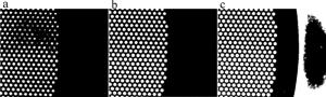
Figure 4. Binarized image
在金属模具表面较为粗糙的情况下,增加膨胀腐蚀的处理,可以提高结果的容错性,方便提取圆轮廓。而且图像二值化之后可能会产生一些微小的像素聚合点,对图像进行膨胀或者腐蚀处理,可以消除这些聚合点,对盲孔边缘进行一定的优化,获得最优图像。
-
边缘跟踪[16-18]可以将检测到的边缘点用某种结构表示出来,方便后续处理。作者使用参考文献[19]中描述的边界追踪算法提取圆轮廓。SUZUKI采用编码的思想,给不同的边界赋予不同的整数值,从而确定它是什么边界以及层次关系。编码遵循两个原则:(1)每次行扫描,遇到以下两种情况,确定外边界和孔边界(f(i, j)表示图片中第i行第j列的密度值):f(i, j-1)=0, f(i, j)=1(outer border); f(i, j)≥1, f(i, j+1)=0(hole border); (2)边界的编号规则。分配一个唯一的标识给新发现的边界,称为边界序列号(number of border,NBD),使用符号B表示。初始时B=1,每次新发现一个边界加1。在这个过程中,遇到f(p, q)=1, f(p, q+1)=0时,将f(p, q)置为-B(f(p, q)表示图片中第p行第q列的边界序列号)。
依照这两个原则,可以将图像中的边界提取出来,并将每一个轮廓以像素点坐标的方式单独存储,得到网点轮廓点的集合。每一个轮廓点的集合都可以用一系列的数据点{(xi, yi)}描述,这些数据点近似地落在一个圆上,根据这些数据可以使用最小二乘法(least squares, LS)估计这个圆的参量。圆的方程可以写为:
$ {\left( {x - {x_{\rm{c}}}} \right)^2} + {\left( {y - {y_{\rm{c}}}} \right)^2} = {R^2} $
(1) 式中, (xc, yc)是圆心坐标,R是半径。展开后有:
$ {x^2} - 2{x_{\rm{c}}}x + x_{\rm{c}}^2 + {y^2} - 2{y_{\rm{c}}}y + y_{\rm{c}}^2 = {R^2} $
(2) 令a=-2xc, b=-2yc, c=xc2+yc2-R2,就可以得到圆的一般方程:
$ {x^2} + {y^2} + ax + by + c = 0 $
(3) 最小二乘法拟合圆需要轮廓点{(xi, yi)}到圆心的距离平方和d最小。d的表达式为:
$ d = \sum {{{\left[ {\sqrt {{{\left( {{x_i} - {x_{\rm{c}}}} \right)}^2} + {{({y_i} - {y_{\rm{c}}})}^2}} - R} \right]}^2}} $
(4) 但是这个方程算起来很麻烦,也得不到解析解。所以退而求其次,简化(4)式得到:
$ \begin{array}{l} d = \sum {{{\left[ {{{\left( {{x_i} - {x_{\rm{c}}}} \right)}^2} + {{\left( {{y_i} - {y_{\rm{c}}}} \right)}^2} - {R^2}} \right]}^2}} = \\ \;\;\;\;\;\;\;\;\sum {{{\left( {x_i^2 + y_i^2 + a{x_i} + b{y_i} + c} \right)}^2}} \end{array} $
(5) 根据最小二乘法的特性,可对上述公式取极值求得参量a,b,c的值,得到下面的条件:
$ \frac{{\partial d}}{{\partial a}} = 0, \frac{{\partial d}}{{\partial b}} = 0, \frac{{\partial d}}{{\partial c}} = 0 $
(6) 即:
$ \left\{ {\begin{array}{*{20}{l}} {\frac{{\partial d}}{{\partial a}} = \sum 2 \left( {x_i^2 + y_i^2 + a{x_i} + b{y_i} + c} \right){x_i} = 0}\\ {\frac{{\partial d}}{{\partial b}} = \sum 2 \left( {x_i^2 + y_i^2 + a{x_i} + b{y_i} + c} \right){y_i} = 0}\\ {\frac{{\partial d}}{{\partial c}} = \sum 2 \left( {x_i^2 + y_i^2 + a{x_i} + b{y_i} + c} \right) = 0} \end{array}} \right. $
(7) 可解得:
$ \left\{ {\begin{array}{*{20}{l}} {a = \frac{{HD - EG}}{{CG - {D^2}}}}\\ {b = \frac{{HC - ED}}{{{D^2} - GC}}}\\ {c = - \frac{{\sum {\left( {x_i^2 + y_i^2} \right)} + a\sum {{x_i}} + b\sum {{y_i}} }}{N}} \end{array}} \right. $
(8) 式中, C=N∑xi2-∑xi∑xi, D=N∑xiyi-∑xi∑yi, E=N∑xi3+N∑xiyi2-∑(xi2+yi2)∑xi, G=N∑yi2-∑yi∑yi, H=N∑yi2+N∑xi2yi-∑(xi2+yi2)∑yi, N表示拟合轮廓点的数量。
至此,就可以求出xc, yc,R的估计拟合值,得到圆心坐标和半径大小:
$ \left\{ {\begin{array}{*{20}{l}} {{x_{\rm{c}}} = - \frac{a}{2}}\\ {{y_{\rm{c}}} = - \frac{b}{2}}\\ {R = \frac{1}{2}\sqrt {{a^2} + {b^2} - 4c} } \end{array}} \right. $
(9) 由此,利用上述方法就可以对提取的圆孔边缘轮廓点进行拟合,精确地得到盲孔的圆心坐标和半径。
-
无论何种匹配算法[20-21],实际上执行的步骤都可以概括为提取特征点,分别获得两幅图片中特征点的坐标和特征点的描述,然后在两幅图片中寻找特征描述,可以把相同的特征点作为匹配点,再以匹配点作为基准进行两幅图片的匹配。本文图片中的特征点即为一个一个白底黑色同样大小的圆,所以就单个圆来说,是不具有足够区分度的特征描述的,能够形成特征的是这些点不同形状的聚合。而这些点的分布都是非常具有规律的等间距六边形密铺,所以网点内部圆的特征点也不是那么明显。基于这两个事实,可以认为需要提取的特征点都在网点的边缘,而特征描述就是这些特征点与其它圆的关系。针对不同的应用场景,特征描述也需要有自己的特性。本文中特征描述主要需要具有平移、旋转、缩放不变性,即一个局部图经过平移、旋转、缩放之后,同一特征点的特征描述在两幅图中应当是不变的。
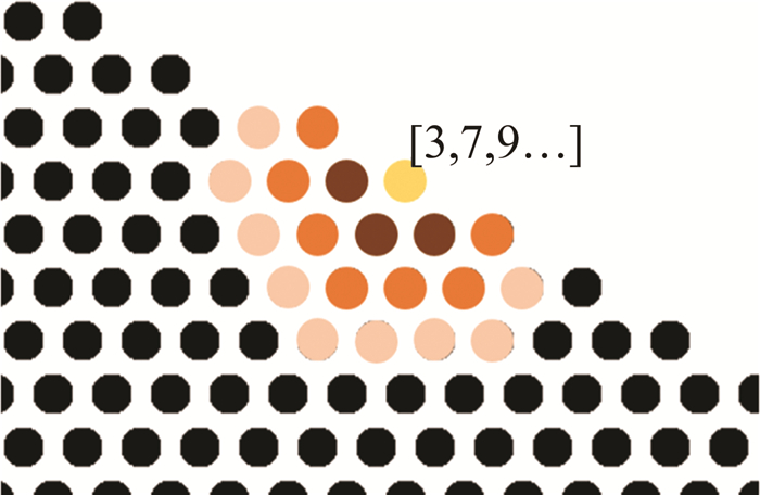
基于以上两个条件,提出了邻域特征法这一特征提取算法,所谓邻域即一个特征点周围的区域内包含的点,邻域中又可以具体划分为不同的阶数,如图 5所示。一个点周围的六边形区域被称为1阶邻域,再往外扩展一个六边形区域,或者说1阶邻域的1阶邻域,邻域的平方称为2阶邻域,以此类推还可以定义3阶邻域、4阶邻域等等。以图 5中有数组标示的圆为例,周围一圈3个圆为1阶邻域,往外一圈7个圆为2阶邻域,再往外一圈9个圆即为3阶邻域。
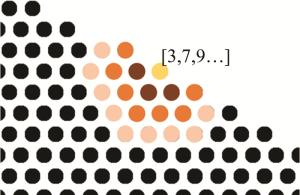
Figure 5. Neighborhood feature of blind holes
在这样的定义下,一个特征点的特征描述就定义为一个数组,数组中的第n个元素就是n阶邻域中圆的数量,特征描述的长度与计算邻域的阶数相同,根据实际情况可以灵活扩充。如果局部图的点数比较少,可以使用较少的阶数,计算更快;局部图点数较多可以多使用几阶,独特性更强。例如图 5中有数组标示的点的3阶特征描述为[3, 7, 9],实际使用的时候,从一个局部图中找到边缘点(特征点),同时剔除距离图片边缘过近的边缘点,这里有一个取舍的判断,假如图片的横向距离大概为15倍的特征点距离,当取5阶特征点的时候左右各需要剔除5个边缘点,这样可供定位的特征点就剩下中间的5个。如果完整图片中圆的数量比较小,可以降低阶数,例如只计算4阶,这样就可以得到7个特征点,如果原始图片中圆的数量比较多,就需要增加阶数,例如计算6阶,只提取3个特征点,理论上来说原图中所有边缘点的信息是被充分利用的。得到特征点之后在原图中计算边缘点相同阶数的特征描述,就可以得到所有特征点的特征描述,匹配的时候依次查找。
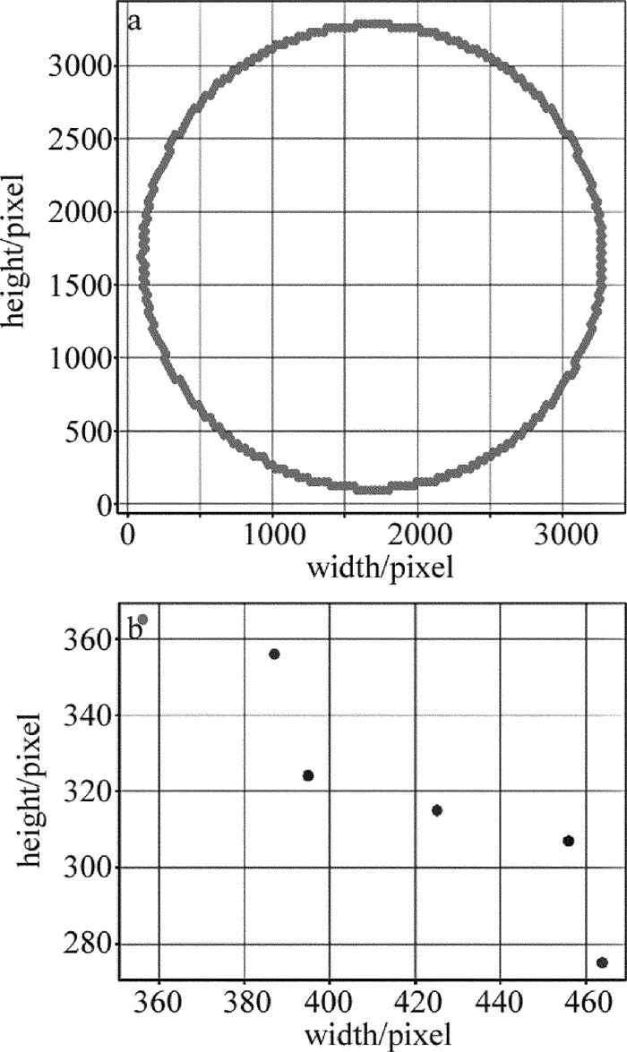
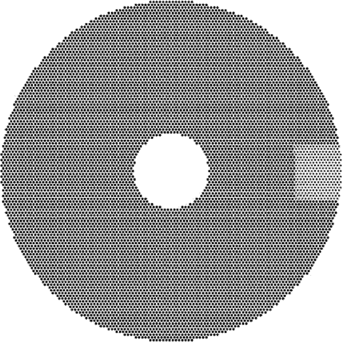
根据理论图的盲孔分布,判断盲孔的1阶邻域内是否存在6个盲孔,提取整个圆盘中盲孔的边缘点分布图,如图 6a所示。以图 5作为研究对象,根据拍摄的局部图识别出的圆心坐标,用相同的方法筛选出局部图的边缘点分布图,如图 6b所示。

Figure 6. Distribution of edge points
根据局部图中边缘点的邻域特征,按照由下至上的顺序逐步寻找其在理论图中的位置,即可锁定局部图在理论图中的位置,实现有效定位,如图 7所示。理论图中只有右上角的部分可以和局部图的特征点完全匹配。
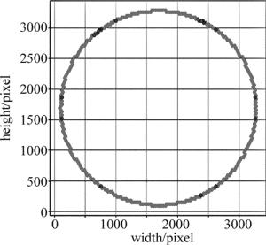
Figure 7. Matching of feature points of local image in theoretical image
匹配完成之后,从局部图和理论图中选出两对对应的特征点,求出两者之间的旋转角和偏移量,就完成了理论图坐标向局部图坐标(平台坐标)的转换,得到理论图中盲孔在平台坐标系中的分布。
-
为验证本算法的基本性能,对分辨率为2464pixel×2056pixel的局部图像进行算法分析。
-
本文中对同一幅图片分别使用霍夫变换和最小二乘法拟合圆检测盲孔,识别效果如图 8所示,检测出的盲孔使用圆圈标注。由图可知,霍夫变换与最小二乘法相比对边缘缺损盲孔的圆心识别精度更高,但是对整体盲孔圆心的识别精度不如最小二乘法。除此之外,霍夫变换对盲孔的识别率低于最小二乘法,会出现部分完整盲孔识别不出的现象,如图 8c所示。最后,使用霍夫变换检测盲孔,如果更换待检测图片就需要手动调参,而最小二乘法不存在这种问题。

Figure 8. a, c—Hough transform b, d—least squares
两种方法识别出盲孔的数量和耗费时间如表 1所示,检测同一幅图片,最小二乘法检测出的盲孔数量更多,是因为边缘缺损盲孔使用最小二乘法更容易检测出来,但圆心精度不高,而且霍夫变换会漏检一些盲孔。两种算法相比,使用最小二乘法的检测速度也更快,效率更高。因此,检测局部图像中的盲孔时,只要设定条件剔除图像边缘的盲孔,同时对图像预处理防止盲孔缺损过大影响识别结果,就可以使用最小二乘法获得最优结果。
Table 1. Comparison of Hough transform and least squares
test 1 test 2 amount time/ms amount time/ms Hough transform 243 424 363 669 least squares 251 115 369 122 由于网点中盲孔在平台坐标的理论位置无法获取,本实验中通过使用激光打标机在平面标刻一个圆,然后将单个圆在平台中移至相机中心,采集图像并使用最小二乘法拟合出其圆心像素坐标,和相机幅面中心坐标(1232, 1028)比较的方式计算整个系统的误差。实验结果得到的系统测量坐标如表 2所示。以系统测量坐标和实际中心坐标(1232,1028)的差值的绝对值作为误差,可计算得到整体平均误差为(0.41,0.34),即圆心位置误差为0.53pixel。依据图 7b对应的实际几何尺寸,计算得到像素尺寸和实际几何尺寸的对应关系是0.016mm/pixel,则系统整体误差为0.008mm。
Table 2. System measurement and error
number measurement/pixel error/pixel 1 (1232.52, 1027.08) (0.52, 0.92) 2 (1232.26, 1027.76) (0.26, 0.24) 3 (1232.85, 1028.81) (0.85, 0.81) 4 (1232.32, 1028.15) (0.32, 0.15) 5 (1231.60, 1027.67) (0.40, 0.33) 6 (1232.33, 1028.40) (0.33, 0.40) 7 (1231.49, 1027.99) (0.51, 0.01) 8 (1231.90, 1027.81) (0.10, 0.19) 9 (1232.31, 1028.36) (0.31, 0.36) 10 (1231.55, 1028.03) (0.45, 0.03) -
依照上述小节邻域特征法的描述,进行实际匹配的结果如图 9所示。采集部分的盲孔使用圆圈标注。邻域特征法依据局部图和整体图的边缘点特征,将两者精确地匹配到一起,匹配时间不超过0.05s。从局部图和理论图中选出两对对应的特征点,可以计算出偏移量和旋转角,据此就可以通过理论图中盲孔的坐标求得盲孔在平台坐标系中的位置。
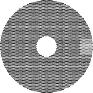
Figure 9. Matching result
采集一张局部图进行匹配时,定位误差会随着相对特征点的距离增大而线性增加,导致计算得到的另一端盲孔圆心位置与实际位置偏差极大。因此,本文中选取两个局部采集图像,在两张局部图中分别选择一个特征点进行计算,求出偏移量、旋转角以及比例系数,使得定位精度得到极大提高,最大误差不超过0.02mm,能够满足实验要求。而使用原始的人工定位方法,定位精度只能达到0.32mm。
-
本文中提出了一种基于最小二乘法拟合和邻域特征法的局部定位整体的网点定位方法。结果表明,本定位方法的定位精度为0.02mm,可以实现对金属滤网盲孔的有效定位。与原始的人工定位方法相比,本定位算法可以极大地缩短工作时间,提高定位精度,对滤网中盲孔实现精准定位。因此,可以在此类金属滤网中推广使用,为在盲孔内的微孔加工提供强有力的基础。
基于邻域特征的网点激光打孔定位算法研究
Research of laser pointing location algorithm based on neighborhood characteristics feature
-
摘要: 为了解决在激光加工中大尺寸多盲孔的网点加工件定位困难的问题, 用工业相机拍摄局部图片, 根据网点中盲孔的结构特征和分布特点, 采用最小二乘法拟合圆的方法检测局部图片中的盲孔, 使用邻域特征的方法寻找网点中的特征点, 并利用特征点匹配实现局部定位整体, 从而实现了加工件的精确和高效定位。结果表明, 邻域特征法对网点中盲孔的定位精度为0.02mm, 实现了对盲孔的有效定位, 解决了网点加工件定位困难的问题。该研究为在盲孔中完成激光加工等后续研究提供了基础。Abstract: In order to solve the difficult problem of locating large size multi-blind holes in laser processing, local pictures were taken by industrial cameras. According to the structure and distribution characteristics of blind holes in meshes, blind holes in local images were detected by least square fitting circle method. Neighborhood feature was used to find feature points in a network. By using feature point matching to realize local localization as a whole, the precise and efficient positioning of the workpiece was realized. The results show that, neighborhood feature method has a positioning accuracy of 0.02mm for blind holes in meshes. Effective positioning of blind holes is realized. It solves the problem of difficult positioning of dot processing parts. This study provides a basis for further research on laser processing in blind holes.
-
Table 1. Comparison of Hough transform and least squares
test 1 test 2 amount time/ms amount time/ms Hough transform 243 424 363 669 least squares 251 115 369 122  下载: 导出CSV
Table 2. System measurement and error
number measurement/pixel error/pixel 1 (1232.52, 1027.08) (0.52, 0.92) 2 (1232.26, 1027.76) (0.26, 0.24) 3 (1232.85, 1028.81) (0.85, 0.81) 4 (1232.32, 1028.15) (0.32, 0.15) 5 (1231.60, 1027.67) (0.40, 0.33) 6 (1232.33, 1028.40) (0.33, 0.40) 7 (1231.49, 1027.99) (0.51, 0.01) 8 (1231.90, 1027.81) (0.10, 0.19) 9 (1232.31, 1028.36) (0.31, 0.36) 10 (1231.55, 1028.03) (0.45, 0.03)
下载: 导出CSV
-
[1] MA X D. Software design of intelligent laser flying processing based on OpenCV visual measurement[D]. Wuhan: Huazhong University of Science and Technology, 2016: 1-5(in Chinese). [2] LI Q. Some research on laser micromachining applied in electronic industry[D]. Hangzhou: Zhejiang University, 2010: 1-23(in Chinese). [3] SUN Sh F, LIAO H P, WU X H, et al. Experimental study about micro hole processing by picosecond laser[J]. Laser Technology, 2018, 42(2):234-238(in Chinese). [4] WEN H, WANG M J, TANG P Sh. An algorithm on graphic joining[J]. Computer Applications and Software, 2000, 17(2):26-29(in Chinese). [5] GUO J. The research of binarization method based on non-uniform illumination images[D]. Wuhan: Wuhan University of Science and Technology, 2013: 5-43(in Chinese). [6] YANG K, ZENG L B, WANG D Ch. A fast arithmetic for the erosion and dilation operations of mathematical morphology[J]. Computer Engineering and Applications, 2005, 41(34):54-56(in Chinese). [7] SHEN X P, PENG G, YUAN Zh Q. Insulator location method based on Hough transformation and RANSAC algorithm[J]. Electronic Measurement Technology, 2017, 40(6):138-143(in Chinese). [8] LIU G Ch, DENG G W. Measurement of geometric characteristics of the electronic component based on OpenCV[J]. Information Technology, 2015(7):165-169(in Chinese). [9] LIU F L, QIAO G F, ZOU B. Precise measurement of circles in industrial computed tomographic images[J]. Optics and Precision Engineering, 2009, 17(11):2842-2848(in Chinese). [10] MAO Q Zh, PAN Zh M, GAO W W. Using iterative hough round transform and connected areato count steel bars reliabley[J]. Geomatic and Information Science of Wuhan University, 2014, 39(3):373-378(in Chinese). [11] XU L. Randomized Hough transform (RHT); basic mechanisms, algorithms, and computational complexities[J]. Cvgip Image Understanding, 1993, 57(2):131-154. doi: 10.1006/ciun.1993.1009 [12] PHILIP K P, DOVE E L, McPHERSON D D, et al. The fuzzy Hough transform-feature extraction in medical images[J]. IEEE Transactions on Medical Imaging, 1994, 13(2):235-240. [13] LIN J L, SHI Q Y. Circle recognition through a point hough transformation[J]. Computer Engineering, 2003, 29(11):17-18(in Ch-inese). [14] AN P Y. Researsh on detection technology of multi-circle workpiece based on machine vision[D]. Hangzhou: Zhejiang Sci-Tech University, 2018: 35-42(in Chinese). [15] YU P, JIANG L X, WANG A Ch, et al. Center of circle detection of the edge missing circle[J]. Geomatics Spatial Information Technology, 2018, 41(7):207-211(in Chinese). [16] ZHANG X Q, WANG J J, JIANG L Y. Circle recognition algorithm based on freeman chain code[J]. Computer Engineering, 2007, 33(15):196-198(in Chinese). [17] CHU G L. Study on the key technologies of automatic identification for cooperative target on spacecraft[D]. Changchun: Changchun Institute of Optics, Fine Mehcanics and Physics, Chinese Academy of Sciences, 2015: 13-30(in Chinese). [18] TANG L L, ZHANG Q C, HU S. An improved algorithm for Canny edge detection with adaptive threshold[J]. Opto-Electronic Engineering, 2011, 38(5):127-132(in Chinese). [19] SUZUKI S, BE K. Topological structural analysis of digitized binary images by border following[J]. Computer Vision Graphics and Image Processing, 1985, 30(1):32-46. doi: 10.1016/0734-189X(85)90016-7 [20] ZHAO L L, GENG G H, LI K, et al. Images matching algorithm based on SURF and fast approximate nearest neighbor search[J]. Application Research of Computers, 2013, 30(3):921-923(in Ch-inese). [21] GAO J, WU Y F, WU K, et al. Image matching method based on corner detection[J]. Chinese Journal of Scientific Instrument, 2013, 34(8):1717-1725(in Chinese). -

 点击查看大图

图(10) / 表(2)
计量
- 文章访问数: 7433
- HTML全文浏览量: 4976
- PDF下载量: 50
- 被引次数: 0
