 网站地图
网站地图


-
高光谱成像技术在不断发展,在军事目标探测、矿物含量检测和农作物成熟度测量等多个领域应用广泛[1]。高光谱的光谱分辨率在不断提高,但是其空间分辨率还不够高,美国机载可见光红外光谱仪[2](airborne visible infrared imaging spectrometer, AVIRIS)采集到的高光谱图像的空间分辨率为20m,较低的空间分辨率使得高光谱在获取图像时,图像中会存在大量的混合像元。对混合像元的解译通常包含端元提取和丰度反演两个部分[3]。高光谱图像中的纯净像元称为端元,寻找端元的过程叫做端元提取;混合像元中各端元的含量称为丰度,利用端元求解混合像元丰度的过程叫做丰度反演[4]。
高光谱的光谱维数较高,在处理数据时,有时需要先对高光谱数据进行降维,使高维数据变为低维数据[5]。高光谱数据的降维方法包括特征提取和波段选择两种[6]。特征提取是对高光谱数据进行投影变换,把数据从高维空间投影到低维空间中,这个过程会破坏光谱曲线的物理意义。波段选择则是从多个波段中选择波段子集,构成低维的光谱空间,从而实现降维。特征提取的典型方法有最小噪声分离[7]和主成分分析[8],波段选择的典型方法主要有最佳指数法和自适应波段选择法[9]等。
线性光谱混合模型认为光谱信号由各端元按照相应的丰度线性组合而成。一般几何上认为,高光谱数据在高维光谱空间中构成凸面单形体,端元分布在凸面单形体的顶点上,而混合像元则主要分布在单形体的内部。近些年,研究者主要从以下算法研究端元提取过程:像元纯度指数、N-FINDR算法、自动目标生成,以及单形体增长算法等。WINTER等人[11]根据最大单形体理论提出了N-FINDR算法,因算法简单易行备受关注。CHANG等人[12]在N-FINDR算法的基础上提出了单形体增长算法,每次增加一个顶点,逐步提取端元。WANG等人[13]采用最小二乘支持向量机的距离尺度计算代替传统N-FINDR算法中的体积计算。XIONG等人[14]通过寻找端元可能的存在区域,减少体积计算过程,提高端元提取速度。
传统的N-FINDR算法利用特征提取的方式对高光谱数据进行降维,使其满足体积公式,但是其破坏了数据的物理意义。为此,本文中利用降维方法中的波段选择代替特征提取方法,其降维后不仅能满足体积公式,而且不改变光谱的物理意义。
-
端元提取时,需要确定端元数目,计算端元数常用的方法有虚拟维度[15]和最小误差高光谱信号识别法(hyperspectral signal identification by minimum error,HYSIME)[16]。本文中用虚拟维度,在一定虚警率下,评估高光谱图像中的端元数P。
-
N-FINDR算法是通过寻找最大体积提取端元,假设高光谱图像中端元的光谱向量为ei=(x1, x2, …, xL)T, i=1, 2, …, P,其中下标L为高光谱的波段数,P为端元数,所有端元组成的光谱矩阵为E=(e1, e2, …, eP)∈RL×P, R代表实数域。首先,利用特征提取方法中的最小噪声分离对高光谱数据降维,使其光谱维度变成P-1维,然后在高光谱图像中选择P个像元点作为初始端元集,最后利用体积公式计算端元集构成的凸面单形体体积[17],体积计算公式为:
$ V(\boldsymbol{E})=\operatorname{abs}(|\boldsymbol{E}|) /(P-1) ! $
(1) $ \mathit{\boldsymbol{E}} = \left[ {\begin{array}{*{20}{c}} 1&1& \cdots &1\\ {{\mathit{\boldsymbol{e}}_1}}&{{\mathit{\boldsymbol{e}}_2}}& \cdots &{{\mathit{\boldsymbol{e}}_P}} \end{array}} \right] $
(2) 式中,|E|为端元矩阵E的行列式,V代表体积,abs为取绝对值,N-FINDR算法将图像中其余的像元点更换其中一个端元,迭代计算其体积,直至找到最大的体积,此公式在计算体积时,需要对高光谱数据降维。GENG等人[18]改进体积公式,使得体积计算不受数据维度限制。令AP-1=[e2-e1, e3-e1, …, eP-e1],变换行列式,则体积公式转换为:
$ \begin{array}{l} \left| {\begin{array}{*{20}{c}} 1&1& \cdots &1\\ {{\mathit{\boldsymbol{e}}_\mathit{\boldsymbol{1}}}}&{{\mathit{\boldsymbol{e}}_2}}& \cdots &{{\mathit{\boldsymbol{e}}_P}} \end{array}} \right| = \\ \left| {\begin{array}{*{20}{c}} 1&0& \cdots &0\\ {{\mathit{\boldsymbol{e}}_1}}&{{\mathit{\boldsymbol{e}}_2} - {\mathit{\boldsymbol{e}}_1}}& \cdots &{{\mathit{\boldsymbol{e}}_P} - {\mathit{\boldsymbol{e}}_1}} \end{array}} \right| = \left| {\begin{array}{*{20}{c}} 1&0\\ {{\mathit{\boldsymbol{e}}_1}}&{{\mathit{\boldsymbol{A}}_{P - 1}}} \end{array}} \right| \end{array} $
(3) $ \begin{array}{c} \left| {\begin{array}{*{20}{c}} 1&1& \cdots &1\\ {{\mathit{\boldsymbol{e}}_1}}&{{\mathit{\boldsymbol{e}}_2}}& \cdots &{{\mathit{\boldsymbol{e}}_P}} \end{array}} \right| = \left| {\begin{array}{*{20}{c}} 1&0\\ {{\mathit{\boldsymbol{e}}_1}}&{{\mathit{\boldsymbol{A}}_{P - 1}}} \end{array}} \right| = \\ \left| {{\mathit{\boldsymbol{A}}_{P - 1}}} \right| = {\left| {{{\left( {{\mathit{\boldsymbol{A}}_{P - 1}}} \right)}^{\rm{T}}}{\mathit{\boldsymbol{A}}_{P - 1}}} \right|^{1/2}} \end{array} $
(4) 由于(AP-1)TAP-1是方阵,因此改进后公式适用于任何维度的高光谱数据,则采用N-FINDR算法时不需要先降维,但是此公式会增加计算量,影响时效性。用特征提取方法降维会破坏像元光谱的物理含义,因此可以考虑用波段选择改进降维方式。同时,波段选择和特征提取降维后都能满足原始的体积计算公式。
-
波段选择也是一种降维方法,波段选择主要依据波段间相关性,信息量及类间可分性[19]。最佳指数法[20](optimal index factor, OIF)是一种经典的波段选择方法,其计算方法简单,且表达的物理意义明确。当用最佳指数法选择k个波段时,计算公式为:
$ S = \frac{{\sum\limits_{i = 1}^k {{\sigma _i}} }}{{\sum\limits_{i = 1}^k {\sum\limits_{j = i + 1}^k {{C_{ij}}} } }} $
(5) 式中, σi为第i波段的标准差,标准差越大,代表波段的信息量越大; Cij为第i波段和第j波段的相关系数,相关系数越小,表示两波段间的相关性越小,则波段间的独立性越好,波段间的信息冗余度越低。利用最佳指数法可以选择出波段中相关性小且信息量大的波段子集,同时实现降维的目的。
本文中将波段选择方法中的最佳指数法引入到N-FINDR算法中,用最佳指数法代替传统N-FINDR算法中的最小噪声分离方法,使降维后不破坏像元的光谱信息,同时提取的端元更加准确,进而使混合像元分解的精度更高。改进的N-FINDR端元提取算法流程如图 1所示。
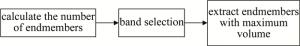
Figure 1. Flow chart of the improved N-FINDR endmember extraction algorithm
由于高光谱数据中端元的真实丰度信息不能准确获得,因此,高光谱混合像元的分解精度一般可通过端元矩阵和丰度矩阵的重构高光谱图像,与原始高光谱图像的均方根误差(root mean square error, RMSE)[21]判别比较,进而判断端元提取的准确性,均方根误差的计算方法为:
$ {M_{{\rm{RUSE}}}} = {\left[ {\frac{1}{n}\sum\limits_{i = 1}^n {{{(\mathit{\boldsymbol{x}} - \mathit{\boldsymbol{\hat x}})}^2}} } \right]^{\frac{1}{2}}} $
(6) 式中, x为原始高光谱图像的像元光谱向量,$ {\mathit{\boldsymbol{\hat x}}}$为解混的端元矩阵和丰度矩阵的重构高光谱图像的像元光谱向量,n为图像中的像元数。MRMSE的值越小,代表端元矩阵和丰度矩阵的重构图像,与原始高光谱图像越相近,说明解混误差越小。
-
本文中用模拟高光谱数据和真实高光谱数据进行实验验证,分别用波段选择方法改进的N-FINDR算法,特征提取的N-FINDR算法和耿修瑞改进的未降维的N-FINDR算法3种方法提取端元,然后用解混方法中常用的全约束最小二乘法解混[22],对比3种方法提取端元的解混精度以及提取端元的时间。
-
模拟高光谱数据采用一种相对简单的模型,从美国地质勘探局光谱库中随机选择4种不同物质的光谱作为端元,实验中所选的4种端元在光谱库中的名称分别为:Dolomite COD2005,Kaolinite CM3,Calcite CO2004和Gibbsite WS214。这4种端元分别用A, B, C和D表示,F是4种光谱的平均值,作为背景。所选端元的波段范围为0.4011μm~2.976μm,波段数目为430。图 2为模拟数据的第50波段灰度图。图 3为所选4种端元的光谱曲线。

Figure 2. Simulation data of the 50th band
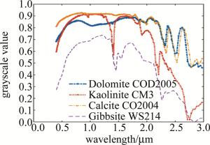
Figure 3. Spectral curves of four endmembers
模拟图像的空间大小为100×100像元,在4行中,每行均有4个大小为15×15像元的方块,其余部分为背景,方块中物质的含量满足“和为1”与“非负”约束,方块的含量如表 1所示。
Table 1. Weight of each endmember in the cube
the 1st column the 2nd column the 3rd column the 4th column the 1st row A 0.75A+0.25B 0.5A+0.5F 0.25A+0.25B+0.5F the 2nd row B 0.75B+0.25C 0.5B+0.5F 0.25B+0.25C+0.5F the 3rd row C 0.75C+0.25D 0.5C+0.5F 0.25C+0.25D+0.5F the 4th row D 0.75D+0.25A 0.5D+0.5F 0.25D+0.25A+0.5F 实际高光谱数据中存在噪声,为使模拟数据更接近真实高光谱数据,选择在模拟数据中加入30dB的高斯噪声。
由于模拟数据中已知实际端元数P=4, 因此需要提取3个波段子集使其满足体积公式,改进的N-FINDR算法利用最佳指数法选择的波段子集为{225, 249, 421}。分别用3种N-FINDR算法提取端元,然后利用全约束最小二乘法解混,解混精度和端元提取时间如表 2所示。
Table 2. RMSE and endmember extraction time of three methods for stimulation data
endmember extraction method the improved N-FINDR algorithm feature extraction N-FINDR algorithm N-FINDR algorithm without dimensionality reduction RMSE 0.0365 0.0385 0.0368 time/s 5.93 8.81 57.89 由表 2可以看出,改进的N-FINDR算法相对其它两种方法的均方根误差都要小,同时可以看到,两种降维之后的N-FINDR算法端元提取时间明显比未降维的N-FINDR算法少。
-
真实高光谱数据采用1997年AVIRIS获取的美国内达华州Cuprite矿区的高光谱图像,从中选择一个100×100像元的子空间进行实验,图 4为所选区域的第50波段的灰度图。高光谱数据的波段范围为0.37μm~2.51μm,将信噪比低的波段98~128和148~170移除,总共利用170个波段进行实验。

Figure 4. Grayscale of the 50th band
改进的N-FINDR算法在虚警率为10-6时,P=4,即端元数为4。用最佳指数法对高光谱数据降维,选择波段子集,波段子集的数目为(P-1),根据公式计算得到的波段子集为{1, 107, 168},此波段子集是相关性小,信息量大的波段,并且满足单形体体积计算公式。特征提取方法的N-FINDR算法是利用最小噪声分离降维,然后根据体积公式计算,选择端元。GENG改进的未降维的N-FINDR算法是改进了体积公式,解决了维数限制,但是也增加了计算量。
3种方法提取端元后,利用全约束最小二乘法解混的均方根误差如表 3所示。由表 3可以看出,利用波段选择方法中的最佳指数法,代替传统N-FINDR算法中最小噪声分离,提取的端元经过解混之后,改进的N-FINDR算法得均方根误差最小,说明改进的N-FINDR算法能有效提取端元,且效果优于传统的N-FINDR算法。
Table 3. RMSE and endmember extraction time of three methods for true data
endmember extraction method the improved N-FINDR algorithm feature extraction N-FINDR algorithm N-FINDR algorithm without dimensionality reduction RMSE 72.63 117.03 107.79 time/s 5.69 5.78 22.93 3种N-FINDR端元提取方法解混后的误差图像如图 5所示。从图中也可以看出, 在绝大多数像元点中,改进的N-FINDR算法比用特征提取方法降维的N-FINDR算法和未降维的N-FINDR算法的误差值小,说明此种改进方法是有效的。
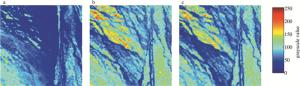
Figure 5. RMSE of three endmember extraction algorithms
通过模拟和真实高光谱数据都能发现,改进的N-FINDR算法的均方根误差比其它两种方法小。同时,降维的N-FINDR算法比未降维的N-FINDR算法端元提取的时间少很多。而且随着光谱数据维度的增加,改进的N-FINDR算法时间会比未降维方法少更多,而且解混精度也相近。
由于改进的N-FINDR算法是利用波段选择降维,其能在满足体积公式的前提下,利用最佳指数法选择相关性小,信息量大的波段,同时不破坏光谱的物理意义,使在端元提取时像元与原始像元更相似,最终提高解混精度,提高算法时效性。
-
高光谱降维方法包括两种方式,特征提取会破坏像元的物理意义,而波段选择则不能破坏其物理意义。将波段选择与N-FINDR算法相结合,代替原本的特征提取方法,在满足体积计算公式的基础上,也不破坏像元光谱曲线的物理含义,使得混合像元的解混精度也得到进一步的提高,说明用波段选择代替特征提取实现高光谱数据的降维,在N-FINDR算法中是可行的。
基于波段选择改进的高光谱端元提取方法
An improved method of hyperspectral endmember extraction based on band selection
-
摘要: 为了解决传统N-FINDR算法降维时破坏像元光谱曲线的物理意义这个问题, 采用波段选择方法中的最佳指数法代替特征提取, 改进N-FINDR算法的降维方式; 利用模拟和真实高光谱数据进行实验, 分别用改进的N-FINDR算法与其它两种算法提取端元, 并用全约束最小二乘法解混。结果表明, 改进的N-FINDR算法的解混精度更高, 用时更少。用波段选择代替特征提取改进降维方式, 保留了光谱曲线的物理意义, 在N-FINDR算法中是可行的。Abstract: In order to solve the problem of destroying the physical meaning of spectral curve of pixels in dimension reduction of traditional N-FINDR algorithm, the best exponential method of band selection was used instead of feature extraction. The dimension reduction method of N-FINDR algorithm was improved. Experiments were carried out using the simulated and real hyperspectral data. The improved N-FINDR algorithm and other two algorithms were used to extract the terminal elements respectively. Full constrained least squares method was used to solve the mixing problem. The results show that the improved N-FINDR algorithm has higher precision and uses less time. It is feasible to use band selection instead of feature extraction to improve the dimension reduction method and retain the physical meaning of spectral curve in N-FINDR algorithm.
-
Key words:
- spectroscopy /
- hyperspectral /
- endmember extraction /
- band selection /
- optimal index factor
-
Figure 5. RMSE of three endmember extraction algorithms
a—improved N-FINDR algorithm b—N-FINDR algorithm with feature extraction c—N-FINDR algorithm without dimensionality reduction
Table 1. Weight of each endmember in the cube
the 1st column the 2nd column the 3rd column the 4th column the 1st row A 0.75A+0.25B 0.5A+0.5F 0.25A+0.25B+0.5F the 2nd row B 0.75B+0.25C 0.5B+0.5F 0.25B+0.25C+0.5F the 3rd row C 0.75C+0.25D 0.5C+0.5F 0.25C+0.25D+0.5F the 4th row D 0.75D+0.25A 0.5D+0.5F 0.25D+0.25A+0.5F  下载: 导出CSV
Table 2. RMSE and endmember extraction time of three methods for stimulation data
endmember extraction method the improved N-FINDR algorithm feature extraction N-FINDR algorithm N-FINDR algorithm without dimensionality reduction RMSE 0.0365 0.0385 0.0368 time/s 5.93 8.81 57.89
下载: 导出CSV
Table 3. RMSE and endmember extraction time of three methods for true data
endmember extraction method the improved N-FINDR algorithm feature extraction N-FINDR algorithm N-FINDR algorithm without dimensionality reduction RMSE 72.63 117.03 107.79 time/s 5.69 5.78 22.93
下载: 导出CSV
-
[1] LIU X. Research of camouflage target detection and evaluation in hyperspectral image [D].Shijiazhuang: Mechanical Engineering College, 2014: 1-2(in Chinese). [2] SHAO T. Research on target recognition in hyperspectral imagery based on spectral information [D]. Harbin: Harbin Institute of Technology, 2010: 4-7(in Chinese). [3] BIONCAS-DIAS J M, PLZAZ A, DOBIGEON N, et al. Hyperspectral unmixing overview: geometrical, statistical, and sparse regression-based approaches[J]. IEEE Journal of Selected Topics Applied Earth Observation and Remote Sensing, 2012, 5(2):354-379. doi: 10.1109/JSTARS.2012.2194696 [4] IORDACHE M D, BIOUCAS-DIAS J M, PLAZA A. Total variation regularization for sparse hyperspectral unmixing[J]. IEEE Transaction Geoscience Remote Sensing, 2012, 50(11):4484-4502. doi: 10.1109/TGRS.2012.2191590 [5] FAN L, LIN X, ALEXANDER W, et al. Feature extraction for hyperspectral imagery via ensemble localized manifold learning [J]. IEEE Geoscience and Remote Sensing Letters, 2015, 12(12): 2486-2490. doi: 10.1109/LGRS.2015.2487226 [6] ZHU G K, HUANG Y C, LEI J S, et al. Unsupervised hyperspectral band selection by dominant set extraction [J]. IEEE Transactions on Geoscience and Remote Sensing, 2016, 54(1):227-619. doi: 10.1109/TGRS.2015.2453362 [7] WANG K, QU H M. Anomaly detection method based on improved minimum noise fraction transformation [J]. Laser Technology, 2015, 39(3):381-385(in Chinese). [8] WANG Q, YANG G, ZHANG J F, et al. Unsupervised band selection algorithm combined with K-L divergence and mutual information [J]. Laser Technology, 2018, 42(3):417-421(in Chinese). [9] LI J, YANG M H, WU K J. Band selection based hyperspectral remote sensing image classification [J]. Journal of Geomatics, 2012, 37(2):41-44(in Chinese). [10] YAN Y, HUA W Sh, LIU X, et al. Research of hyperspectral unmixing methods[J].Laser Technology, 2018, 42(5):692-698(in Chinese). [11] WINTER M E. N-FINDR: an algorithm for fast autonomous spectral endmember determination in hyperspectral data[J].Proceedings of the SPIE, 1999, 3753:266-275. doi: 10.1117/12.366289 [12] CHANG C I, WU C C, LIU W M. A new growing method for simplex-based endmember extraction algorithm [J]. IEEE Transaction on Geoscience and Remote Sensing, 2006, 44(10):2804-2819. doi: 10.1109/TGRS.2006.881803 [13] WANG L G, DENG L Q, ZHANG J. Endmember selection algorithm based on linear least square support vector machines[J].Spectroscopy and Spectral Analysis, 2010, 30(3): 743-747 (in Ch-inese). [14] XIONG W, CHANG C I, WU C C. Fast algorithms to implement N-FINDR for hyperspectral endmember extraction[J].IEEE Journal of Selected Topics in Applied Earth Observation and Remote Sensing, 2011, 4(3):545-564. doi: 10.1109/JSTARS.2011.2119466 [15] CHANG C I, DU Q. Estimation of number of spectrally distinct signal in hyperspectral imagery [J].IEEE Transactions on Geoscience and Remote Sensing, 2004, 42(3):608-619. doi: 10.1109/TGRS.2003.819189 [16] MARTIN G, PLAZA A. Region-based spatial preprocessing for endmember extraction and spectral unmixing [J]. IEEE Transaction on Geoscience and Remote Sensing, 2011, 8(4):745-749. doi: 10.1109/LGRS.2011.2107877 [17] YAN Y, HUA W Sh, CUI Z H, et al. Classification volume for hyperspectral endmember extraction[J]. Laser Optoelectronics Progress, 2018, 55(9):093004(in Chinese). doi: 10.3788/LOP [18] GENG X, ZHAO Y, WANG F, et al. A new volume formula for a simplex and its application to endmember extraction for hyperspectral image analysis [J]. International Journal of Remote Sensing, 2010, 31(4):1027-1035. doi: 10.1080/01431160903154283 [19] GONG W J, DONG A G, HAN X. Band selection algorithm for hyperspectral images based on band index [J]. Laser Technology, 2017, 41(4):507-510(in Chinese). [20] REN X D, LEI W H, GU Y, et al. Improved band selection method for hyperspectral imagery [J]. Computer Science, 2015, 42(11): 162-168(in Chinese). [21] PLAZA A, PABLO M, ROSA P, et al. A quantitative and comparative analysis of endmember extraction algorithms from hyperspectral data [J]. IEEE Transactions on Geoscience and Remote Sensing, 2004, 42(3):650-663. doi: 10.1109/TGRS.2003.820314 [22] DANIEL C H, CHEIN I C. Fully constrained least squares linear spectral mixture analysis method for material quantification in hyperspectral imagery [J]. IEEE Transaction on Geoscience and Remote Sensing, 2001, 39(3):529-545. doi: 10.1109/36.911111 -

 点击查看大图

图(5) / 表(3)
计量
- 文章访问数: 5796
- HTML全文浏览量: 4057
- PDF下载量: 20
- 被引次数: 0
