 网站地图
网站地图

 下载:
下载:


-
调频连续波(frequency modulated continuous wave, FMCW)激光雷达具有大带宽、高精度、高测量分辨力等优点,广泛应用于各种非接触式测量领域[1-2]。其基本原理是对发射激光的频率进行线性调制,本振信号与回波信号干涉形成拍频信号,通过提取拍频信号中的频率信息来计算测量距离[3]。实际测量时,激光器存在调制非线性问题,造成测量信号频谱展宽严重,使得调频连续波测距系统的测距精度受到很大限制[4-6]。
为解决这一问题,学者们提出了很多有效的方法,主要有主动补偿与后处理两大类技术。主动补偿主要有预校正补偿及反馈调频技术、电光锁相环反馈校正技术等[7-8]。后处理技术有分子频率参考校正、光频梳校正、双光路校正等方法[9-11]。其中双光路校正技术结构简单、装置易于搭建,常用方法为双光路零点重采样法,该方法有两路干涉光路,而辅助干涉光路产生的拍频信号也包含有非线性信息,提取辅助干涉光路的拍频信号零点位置点对测量光路拍频信号对应位置点进行采样处理,以达到消除非线性的目的。但是在利用双干涉光路进行采样的过程中,为了满足奈奎斯特采样定律,需要保证时钟信号频率至少为被采样信号的两倍,这是这种方法的缺陷,因为要保证辅助干涉光路的光程差至少要大于两倍的测量距离。进行大长度测量时,所需辅助干涉光路的参考延时光纤将会更长,受环境振动以及光纤色散等问题的影响将会越来越大,需要严格控制参考光纤的温度、湿度、偏振态以及进行色散补偿。哈尔滨工业大学的XU等人研究了振动、色散等因素对于调频连续波测距的影响,并基于希尔伯特变换对信号进行移相来增加测量受限距离[12-14]。天津大学PAN等人分析了色散对于等光频重采样测距精度的影响并对色散进行了校正,还研究了多重信号特性算法用于估计均方根误差,并提出了精度评定方法[15-17]。日本金泽大学的IIYAMA等人提出了利用电子锁相环对辅助干涉光路拍频信号进行倍频的方法,对辅助拍频信号倍频后,可以利用短的参考延时光路对长距离测量信号进行重采样解决非线性问题,但是这种方法加入了倍频系统,使得测量分辨力与精度也会受到倍频精度的影响,引入了额外的误差,大大增加了系统成本与复杂度[18]。
本文中在双光路校正技术的基础上,提出了等光频细分重采样法来消除激光器调制非线性的影响,对等光频细分重采样算法进行了详细的推导,通过仿真验证了公式的正确性,结合算法搭建相应短光纤辅助测距光路进行等光频细分重采样系统测距能力的实验验证,实现了利用短光纤对长距离测量信号重采样。
-
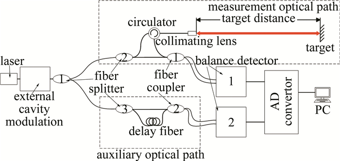
等光频细分重采样系统的测量原理及光路结构如图 1所示。系统采用双光路结构,由两路并联的马赫-曾德尔干涉光路组成,一路为作为测量干涉光路,另外一路作为辅助干涉光路。
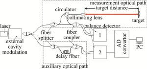
Figure 1. Optical structure diagram of laser ranging system of equal optical frequency subdivision resampling
系统主要由光纤光路构成,光纤采用单模光纤,激光通过第1个80:20光纤分束器1后分为两束光,能量较高一束进入测量干涉光路部分,保证探测回波信号能量足够与本振信号形成信噪比较高的拍频信号;另一束进入辅助干涉光路部分。进入测量干涉光路部分的光再经过分束器2分为出射测量光与本振光,出射测量光通过光纤环形器及准直透镜发射向待测目标镜,反射回光通过环形器再与测量干涉光路本振光在耦合器1处发生干涉;另一束进入辅助干涉光路部分经过分束器3分为两束,一路经过已知长度的短参考光纤后与另一路辅助干涉光路本振光发生干涉。
激光器发出的扫频激光电场强度可以表示为:
$ E(t) = A(t)\cos \left( {\omega t - {\varphi _0}} \right) $
(1) 式中, A(t)表示电场振幅随时间变化值,由于激光器频率调制的过程中伴随有非自主的幅度调制,所以激光电场振幅大小是随时间不断变化的,但是对相位计算并不影响,故可看作恒定值A0,ω为调频激光器出射激光的电场角频率,φ0为初始相位。
由欧拉公式可以得到出射激光电场强度指数形式的表达式为:
$ E(t) = {A_0}{{\rm{e}}^{{\rm{i}}\varphi (t)}} $
(2) 式中, φ(t)为瞬时相位,为扫频激光器出射激光瞬时角频率ω(t)在时间t的积分:
$ \varphi (t) = \int_0^t \omega (t){\rm{d}}t + {\varphi _0} $
(3) 扫频激光器出射激光瞬时角频率为:
$ \omega (t) = \mathit{\Omega }t + {\omega _0} $
(4) 式中, ω0为扫频初始角频率,Ω为激光器扫频角频率的变化率,理论上Ω=4πB0/T,其中B0为扫频带宽,T为扫频周期,实际中扫频角频率变化率不是固定不变的,导致了扫频非线性问题。
将(3)式、(4)式代入(2)式得:
$ E(t) = {A_0}\exp \left[ {{\rm{i}}\left( {\frac{1}{2}\mathit{\Omega }{t^2} + {\omega _0}t + {\varphi _0}} \right)} \right] $
(5) 扫频激光器出射激光分为两路, 分别进入辅助干涉光路部分与测量干涉光路部分,进入辅助干涉光路部分激光由分束器3分为两束分别进入辅助干涉光路俩臂,由于辅助干涉光路两臂之间存在光程差,导致两路激光在耦合器2处存在时间延迟,在耦合器2处辅助干涉光路测量臂及参考臂对应的电场强度分别为:
$ \left\{ \begin{array}{l} \begin{array}{*{20}{c}} {{E_{{\rm{AM}}}}(t) = {A_{{\rm{AM}}}}\exp \left\{ {{\rm{i}}\left[ {\frac{1}{2}\mathit{\Omega }{{\left( {t - {\tau _{\rm{a}}}} \right)}^2} + } \right.} \right.}\\ {\left. {\left. {{\omega _0}\left( {t - {\tau _{\rm{a}}}} \right) + {\varphi _0}} \right]} \right\}} \end{array}\\ {E_{{\rm{AR}}}}(t) = {A_{{\rm{AR}}}}\exp \left\{ {{\rm{i}}\left[ {\frac{1}{2}\mathit{\Omega }{t^2} + {\omega _0}t + {\varphi _0}} \right]} \right\} \end{array} \right. $
(6) 式中, τa为辅助干涉光路两臂时间延迟,AAM为辅助干涉光路测量臂信号幅值,AAR为辅助干涉光路参考臂信号幅值。
辅助干涉光路两臂信号在探测器2处叠加电场光强变化为电场复振幅与共轭的乘积:
$ {I_{\rm{a}}}(\tau ,t) = \left( {{E_{{\rm{AR}}}} + {E_{{\rm{AM}}}}} \right) \cdot \left( {E_{{\rm{AR}}}^* + E_{{\rm{AM}}}^*} \right) $
(7) 由于探测器无法探测到叠加高频信息,探测器2处仅探测到光强拍频信号,可以表示为:
$ \begin{array}{*{20}{c}} {{I_{\rm{a}}}\left( {{\tau _{\rm{a}}},t} \right) = {I_{{\rm{AR}}}} + {I_{{\rm{AM}}}} + }\\ {2\sqrt {{I_{{\rm{AR}}}}{I_{{\rm{AM}}}}} \cos \left[ {{\varphi _{{\rm{AR}}}}(t) - {\varphi _{{\rm{AM}}}}(t)} \right] = }\\ {{I_{{\rm{a}},0}}\left[ {1 + {V_{\rm{a}}}\cos \left( {\mathit{\Omega }{\tau _{\rm{a}}}t + {\omega _0}{\tau _{\rm{a}}} + \frac{1}{2}\mathit{\Omega }\tau _{\rm{a}}^2} \right)} \right]} \end{array} $
(8) 式中, IAR为辅助干涉光路参考臂信号光强,IAM为辅助干涉光路测量臂信号光强,φAR(t)为辅助干涉光路参考臂瞬时相位,φAM(t)为辅助干涉光路测量臂瞬时相位,Ia, 0为辅助干涉光路平均光强,Va表示辅助干涉光路光电探测器表面幅值。公式中最后一项为光程差时延对应的2阶小量,由于等光频细分重采样法所需的辅助光路光程很短,所以此项可以忽略不计,辅助拍频信号公式即可表示为:
$ {I_{\rm{a}}}\left( {{\tau _{\rm{a}}},t} \right) = {I_{{\rm{a}},0}}\left[ {1 + {V_{\rm{a}}}\cos \left( {\mathit{\Omega }{\tau _{\rm{a}}}t + {\omega _0}{\tau _{\rm{a}}}} \right)} \right] $
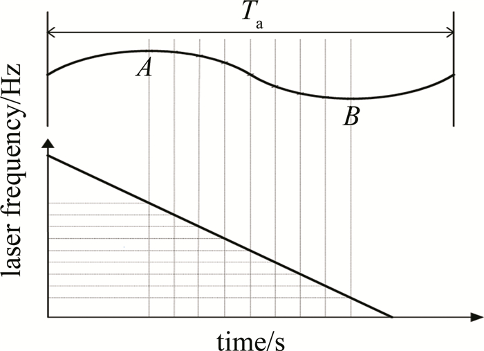
(9) 如图 2所示,首先提取辅助干涉光路产生的拍频信号峰谷值点作为特征点,特征点携带有不断变化的非线性信息。
峰值特征点A点拍频相位为:
$ {\varphi _A} = {\mathit{\Omega }_A}{\tau _{\rm{a}}}{t_A} + {\omega _0}{\tau _{\rm{a}}} = 2{\rm{ \mathsf{ π} }}m $
(10) 谷值特征点B点拍频相位为:
$ {\varphi _B} = {\mathit{\Omega }_B}{\tau _{\rm{a}}}{t_B} + {\omega _0}{\tau _{\rm{a}}} = 2{\rm{ \mathsf{ π} }}\left( {m + \frac{1}{2}} \right) $
(11) 式中, φA, φB分别为A, B两点的瞬时相位; tA, tB分别为
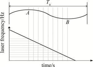
Figure 2. Schematic diagram of equal optical frequency subdivision of auxiliary beat signal
A, B两点对应的实际时间; ΩA, ΩB为A, B两点对应的实时角频率变化率; m表示峰谷值特征点A, B在辅助拍频信号的第m个周期。
所以A, B两点之间的拍频相位差为:
$ \Delta {\varphi _{A,B}} = {\varphi _B} - {\varphi _A} = {\rm{ \mathsf{ π} }} $
(12) 对应的A, B两点之间的激光角频率差为:
$ \Delta {\omega _{A,B}} = \frac{{\Delta {\varphi _{A,B}}}}{{{\tau _{\rm{a}}}}} = \frac{{\rm{ \mathsf{ π} }}}{{{\tau _{\rm{a}}}}} $
(13) 将辅助拍频信号特征点之间的半个拍频周期细化为N段等时间间隔段,两相邻间隔点之间的时间间隔即为Ta/(2N),Ta为一个辅助拍频信号的周期长度。在相邻特征点之间,扫频频率非线性变化对辅助干涉光路拍频信号影响很小,特征点之间扫频频率变化具有局部线性,特征点之间的半个周期内等时间间隔点对应的等光频间隔点,结合(13)式可得相邻间隔点之间的对应激光角频率差为:
$ \Delta \omega = \frac{{\rm{ \mathsf{ π} }}}{{N{\tau _{\rm{a}}}}} $
(14) 由于辅助干涉光路光程差长度不变,τa为恒定值,所以辅助拍频信号间隔点之间对应的激光角频率间隔恒为π/(Nτa)。
测量干涉光路拍频信号表达式与辅助干涉光路拍频信号表达式推导过程相同,测量拍频信号Im可以表示为:
$ {I_{\rm{m}}}\left( {{\tau _{\rm{m}}},t} \right) = {I_{{\rm{m}},0}}\left[ {1 + {V_{\rm{m}}}\cos \left( {\mathit{\Omega }{\tau _{\rm{m}}}t + {\omega _0}{\tau _{\rm{m}}}} \right)} \right] $
(15) 式中, Im, 0为测量干涉光路平均光强,Vm表示测量干涉光路光电探测器表面幅值,τm为测量干涉光路两臂时间延迟。
利用等光频细分后的辅助拍频信号点作为时钟信号采样测量拍频信号,使得重采样后的测量拍频信号点之间同样满足等光频间隔关系,重采样后的测量信号将不再以时间间隔而以光频间隔π/(Nτa)为基本单位,将原有的等时间间隔采样转化为等频率间隔采样,进行等光频细分重采样后的测量拍频信号Im可以表示为:
$ \begin{array}{*{20}{c}} {{I_{\rm{m}}}\left( {{\tau _{\rm{m}}},k} \right) = {I_{{\rm{m}},0}}\left[ {1 + {V_{\rm{m}}}\cos \left( {\frac{{{\rm{ \mathsf{ π} }}{\tau _{\rm{m}}}}}{{N{\tau _{\rm{a}}}}}k + {\omega _0}{\tau _{\rm{m}}}} \right)} \right],}\\ {\left( {k = 0,1,2, \cdots } \right)} \end{array} $
(16) 对等光频细分重采样后的测量拍频信号进行快速傅里叶变换(fast Fourier transform, FFT)[19]得到测量干涉光路两臂时间延迟:
$ {\tau _{\rm{m}}} = \frac{{2N{P_{\max }}}}{M}{\tau _{\rm{a}}} $
(17) 式中, Pmax为FFT频谱的峰值位置,M为总FFT点数。
可以得到测量距离公式为:
$ D = \frac{{c{\tau _{\rm{m}}}}}{2} = \frac{{N{L_{\rm{a}}}{P_{\max }}}}{M} $
(18) 式中, c为光速,La为辅助干涉光路两臂之间的光程差。
等光频细分重采样系统允许测得的最大范围与细分段数N成正比:
$ {D_{\max }} < \frac{N}{2}{L_{\rm{a}}} $
(19) 由(19)式可知,等光频细分重采样系统可以通过增多细分段数N的方式减少所需辅助干涉光路光程差La的长度,所以等光频细分重采样系统可使用较短的辅助参考光纤, 代替原有双光路零点重采样系统所必需的长参考光纤,理论上细分段数的上限值受到原始数据采集频率的限制,须保证细分后间隔点不重叠。
-
为验证重新推导得出的等光频细分重采样频谱分析公式的正确性,在这里以多项式信号作为调频非线性拍频信号的主要形式进行仿真验证。
设扫频激光器调制范围为1543.7nm~1553.7nm,扫频速度预设为100nm/s, 则激光器调制频率变化率为:
$ \begin{array}{*{20}{c}} {\mathit{\Omega } = 12508095395690 \times }\\ {[1 + 0.001 \times \sin (2000{\rm{ \mathsf{ π} }} \times t)]} \end{array} $
(20) 式中,0.001×sin(2000π×t)项为调制频率变化率非线性波动干扰项,实际波动范围以及频率要小于此,为验证等光频细分重采样法的处理能力,将波动范围及波动频率增大。
预设测量距离为9m,辅助干涉光路光程差为5m,测量距离大于辅助干涉光路光程差的1/2,辅助拍频信号可以表示为:
$ \begin{array}{*{20}{c}} {{S_{\rm{a}}} = 6 \times \cos (2{\rm{ \mathsf{ π} }} \times \mathit{\Omega } \times t \times 5/c + }\\ {193087468623286 \times 5/c)} \end{array} $
(21) 测量拍频信号可以表示为:
$ \begin{array}{*{20}{c}} {{S_{\rm{m}}} = 8 \times \cos (2{\rm{ \mathsf{ π} }} \times \mathit{\Omega } \times t \times 18/c + }\\ {193087468623286 \times 18/c)} \end{array} $
(22) 仿真结果如图 3所示。采样点数设置为90万个点,采样频率为25MHz,用辅助拍频信号Sa对测量拍频信号Sm进行等光频细分重采样后,进行100倍补零FFT运算,得到FFT频谱的峰值位置点为2701306,总FFT点数为6002900,等光频细化段数N为4段,保证理论允许的最大测量范围大于实际范围,代入(16)式得到仿真距离:
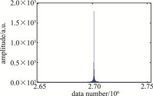
Figure 3. Spectral diagram of the simulated signal after equal optical frequency subdivision resampling
$ {D_{{\rm{sim}}}} = \frac{{N{L_{\rm{a}}}{P_{{\rm{max}}}}}}{M} = \frac{{4 \times 5 \times 2701306}}{{6002900}} = 9.000003 $
(23) 求得仿真距离为9.000003m,由于离散化误差的影响,造成结果存在细微偏差。
-
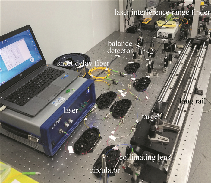
为验证等光频细分重采样系统测距能力以及对调制非线性的消除效果,按照图 1系统搭建了实验装置, 如图 4所示。实验中使用的是Luna PHOENIX 1400可调谐激光器,调制范围设置为1540nm~1560nm,调制速度为100nm/s;测量光路从准直透镜出射到空间测量光路之前存在固有光纤光路长度3.2m;辅助干涉光纤长度为2.104m,辅助干涉光路长度小于测量距离的2倍;待测目标镜放置于带有激光干涉仪(Re-nishawXL-80)的1m长导轨上,由近到远移动目标镜的位置,移动步长为100mm;示波器采样频率为25MHz,使用设计的等光频细分重采样测距系统对目标镜的距离进行测量。

Figure 4. Experimental device diagram
如图 5所示,其中实线部分为等光频细分重采样系统辅助干涉光路产生的辅助拍频信号,其中圆形点表示等光频细分处理辅助拍频信号后得到的等光频间隔时钟信号点位置,细分段数N=8,虚线部分为测量拍频信号,其中叉状点表示等光频间隔时钟信号点对测量信号重采样后的位置点。由于辅助干涉光路光程长度小于测量光路光程长度,造成参考信号频率小于测量信号频率。如果直接对短距离参考光路辅助干涉光路拍频信号提取零点位置对测量信号进行重采样,将使重采样后的信号严重失真,使用等光频细分重采样算法后,辅助拍频信号每个周期的可用重采样时钟信号点数增加,使得重采样过程可以满足奈奎斯特采样定理。
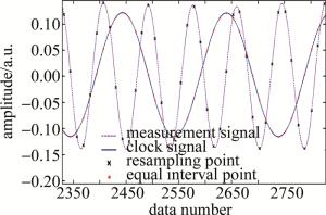
Figure 5. Comparison of clock signal and measurement signal waveforms of equal optical frequency subdivision resampling system
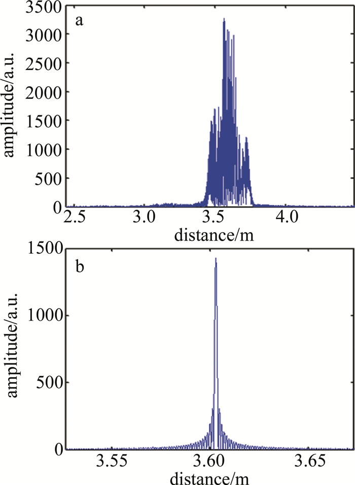
对比图 6两小图可以看出,图 6a中, 由于激光器调制非线性的影响,对测量拍频信号直接进行FFT后的频谱发生了严重展宽,无法识别出准确的距离信息,测量分辨力也极大地下降;图 6b中,经过等光频细分重采样后的测量信号频谱可以准确地识别出测量信号中的距离信息,半峰全宽接近理论分辨力的大小,证明了等光频细分重采样有效地抑制了激光器的调制非线性的影响。

Figure 6. Comparison of nonlinear cancellation effects of the measured beat signal a—before equal optical frequency subdivision resampling b—after equal optical frequency subdivision resampling
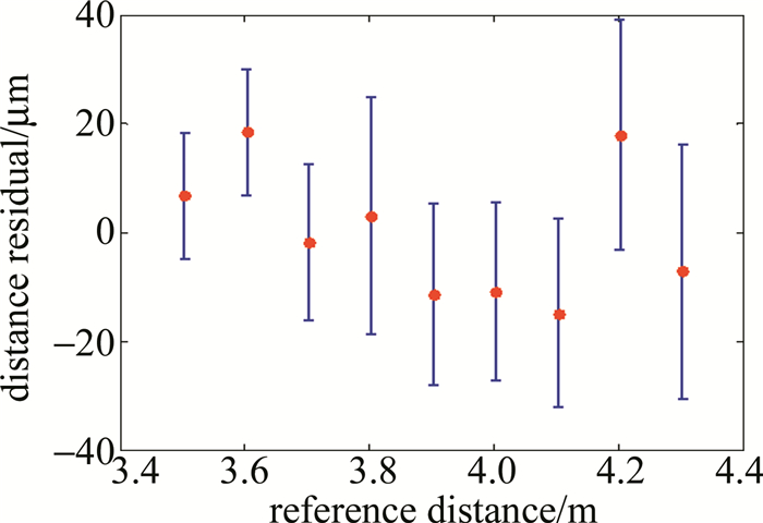
如图 7所示,在实验室环境下,在绝对距离4.3m(其中包含固有光纤光路长度)测量范围内,等光频细分重采样测距系统测量值与激光干涉仪距离变化值相比最大残余误差小于±18.46μm,最大标准差为22.23μm。此误差主要来源于如下几个方面:测量光路信号本身存在环境振动的影响,如位移台的抖动,光学支撑器件的振动放大以及测量光路光纤光路部分存在的环境振动,细微振动造成的多普勒频移导致傅里叶变换后的频谱发生展宽和漂移使得测量精度降低;激光干涉仪本身也存在测量标准差;等光频细分重采样测距系统与激光干涉仪出射光并不能完全在一条直线上,存在一定夹角造成阿贝误差。
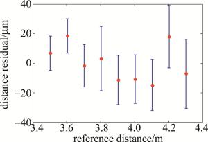
Figure 7. Distance residuals compared with laser interferometer within 4.3m
-
在双光路校正技术的基础上提出了等光频细分重采样法,并对此方法进行了详细的推导,该方法可以通过对特征峰谷值点之间信号段进行等光频细分,以增加辅助干涉拍频信号时钟信号点的提取数量,消除调制非线性的同时,降低了对辅助光路长度的要求。实验结果表明:等光频细分重采样系统在100nm/s的调节速度以及20nm的带宽时,对4.3m测量范围的待测目标镜进行测量,使用等光频细分重采样法对信号进行处理后,测量结果与激光干涉仪相比的最大残余误差在±18.46μm之间,最大测量标准差为22.23μm。实验结果验证了本文中理论分析的可行性,等光频细分重采样的方法有效地抑制了激光器的调制非线性的影响。通过多个位置处的重复测距实验表明,该方法有较高的单点稳定性与测距准确度。
基于等光频细分重采样的调频干涉测距方法
Laser ranging method of frequency modulation interference based on equal optical frequency subdivision resampling
-
摘要: 为了解决调频连续波(FMCW)激光器调制非线性导致的测量信号频谱展宽降低激光干涉测距精度的问题, 采用一种基于等光频细分重采样的调频干涉测距方法, 进行了理论分析和实验验证, 获得了双光路测距系统对不同位置目标信号等光频细分重采样后的波形数据, 并进行了频谱分析。结果表明, 通过等光频细分重采样的方法, 使用细分后的时钟信号点对距离大于辅助干涉光路光程差的目标测量信号进行重采样, 消除了激光器的调制非线性的影响, 并且避免了采样点数不足引起信号失真的问题; 在4.3m测量范围内, 等光频细分重采样测距系统与激光干涉仪相比最大残余误差不超过±18.46μm, 最大测量标准差为23.39μm; 该方法使用的辅助干涉光路光程差很短, 受环境的影响较小, 可以获得稳定的时钟信号, 并且可以减少双光路FMCW测距系统的体积与成本。该研究为长距离、高精度调频连续波测量提供了实用参考。Abstract: In order to solve the problem that modulation nonlinearity of frequency modulated continuous wave(FMCW) laser leads to the broadening of measurement signal spectrum and the reduction of laser interferometric ranging accuracy, frequency modulated interferometry ranging method based on equal optical frequency subdivision and resampling was adopted. Theoretical analysis and experimental verification were carried out. Waveform data of dual optical path ranging system after equal optical frequency subdivision and resampling of target signals at different positions were obtained. Spectrum analysis was also carried out. The results show that, by means of equal optical frequency subdivision and resampling, the subdivided clock signal points are used to resample the target measurement signal whose distance is greater than optical path difference of auxiliary interferometer. The influence of modulation nonlinearity of laser is eliminated. The problem of signal distortion caused by insufficient sampling points is avoided. Within the measurement range of 4.3m, comparing with laser interferometer, the maximum residual error of equal optical frequency subdivision resampling ranging system does not exceed ±18.46μm. The maximum standard deviation is 23.39μm. Optical path difference of auxiliary interferometer used in this method is very short. It is less affected by the environment. A stable clock signal can be obtained. It can also reduce the volume and cost of dual optical path FMCW ranging system. This study provides practical reference for long-distance and high-precision FMCW measurement.
-
Figure 1. Optical structure diagram of laser ranging system of equal optical frequency subdivision resampling
Figure 2. Schematic diagram of equal optical frequency subdivision of auxiliary beat signal
Figure 3. Spectral diagram of the simulated signal after equal optical frequency subdivision resampling
Figure 5. Comparison of clock signal and measurement signal waveforms of equal optical frequency subdivision resampling system
Figure 6. Comparison of nonlinear cancellation effects of the measured beat signal a—before equal optical frequency subdivision resampling b—after equal optical frequency subdivision resampling
-
[1] MATEO A B, BARBER Z W. Multi-dimensional, non-contact metrology using trilateration and high resolution FMCW ladar[J]. Applied Optics, 2015, 54(19): 5911-5916. doi: 10.1364/AO.54.005911 [2] DILAZARO T, NEHMETALLAH G. Large-volume, low-cost, high-precision FMCW tomography using stitched DFBs[J]. Optics Express, 2018, 26(3): 2891-2904. doi: 10.1364/OE.26.002891 [3] KAKUMA S. Frequency-modulated continuous-wave laser radar using dual vertical-cavity surface-emitting laser diodes for real-time mea-surements of distance and radial velocity[J]. Optical Review, 2017, 24(1): 39-46. doi: 10.1007/s10043-016-0294-7 [4] ZHANG T, QU X H, ZHANG F M. Nonlinear error correction for FMCW ladar by the amplitude modulation method[J]. Optics Express, 2018, 26(9): 11519-11528. doi: 10.1364/OE.26.011519 [5] ZHANG Y Y, GUO Y, REN Y J, et al. Study of drift error and its compensation method in absolute distance measurement by optical frequency scanning interferometry[J]. Acta Optica Sinica, 2017, 37(12): 1212001(in Chinese). [6] JI N K, ZHANG F M, QU X H, et al. Ranging technology for frequency modulated continuous wave laser based on phase difference frequency measurement[J]. Chinese Journal of Lasers, 2018, 45(11): 1104002(in Chinese). doi: 10.3788/CJL201845.1104002 [7] ROOS P A, REIBEL R R, BERG T, et al. Ultrabroadband optical chirp linearization for precision metrology applications[J]. Optics Letters, 2009, 34(23): 3692-3694. doi: 10.1364/OL.34.003692 [8] BEHROOZPOUR B, SANDBORN P A M, QUACK N, et al. Elec- tronic-photonic integrated circuit for 3-D microimaging[J]. IEEE Journal of Solid-State Circuits, 2017, 52(1): 161-172. doi: 10.1109/JSSC.2016.2621755 [9] MATEO A B, BARBER Z W. Precision and accuracy testing of FMCW ladar-based length metrology[J]. Applied Optics, 2015, 54(19): 6019-6024. doi: 10.1364/AO.54.006019 [10] BAUMANN E, GIORGETTA F R, CODDINGTON I, et al. Comb-calibrated frequency-modulated continuous-wave ladar for absolute distance measurements[J]. Optics Letters, 2013, 38(12): 2026-2028. doi: 10.1364/OL.38.002026 [11] SHI G, ZHANG F M, QU X H, et al. High-resolution frequency-modulated continuous-wave laser ranging for precision distance metrology applications[J]. Optical Engineering, 2014, 53(12): 122402. doi: 10.1117/1.OE.53.12.122402 [12] XU X K. Research on key technologies of laser frequency scanning interference absolute distance measurement[D]. Harbin: Harbin Institute of Technology, 2017: 36-53(in Chinese). [13] XU X K, LIU G D, LIU B G, et al. Research on the fiber dispersion and compensation in large-scale high-resolution broadband frequency-modulated continuous wave laser measurement system[J]. Optical Engineering, 2015, 54(7): 074102. doi: 10.1117/1.OE.54.7.074102 [14] LIU G D, XU X K, LIU B G, et al. Dispersion compensation method based on focus definition evaluation functions for high-resolution laser frequency scanning interference measurement[J]. Optics Communications, 2017, 386: 57-64. doi: 10.1016/j.optcom.2016.10.052 [15] PAN H, ZHANG F M, SHI Ch Zh, et al. High-precision frequency estimation for frequency modulated continuous wave laser ranging using the multiple signal classification method[J]. Applied Optics, 2017, 56(24): 6956-6961. doi: 10.1364/AO.56.006956 [16] PAN H, QU X H, SHI Ch Zh, et al. Precision evaluation method of measuring frequency modulated continuous wave laser distance[J]. Acta Physica Sinica, 2018, 67(9): 090201(in Chinese). [17] PAN H, QU X H, SHI Ch Zh, et al. Resolution-enhancement and sampling error correction based on molecular absorption line in frequency scanning interferometry[J]. Optics Communications, 2018, 416: 214-220. doi: 10.1016/j.optcom.2018.02.006 [18] IIYAMA K, YASUDA M, TAKAMIYA S. Extended-range high-re-solution FMCW reflectometry by means of electronically frequency-multiplied sampling signal generated from auxiliary interferometer[J]. IEICE Transactions on Electronics, 2006, 89(6): 823-829. [19] ZHU L K, JIA F X, LI X L. Design of parallel high-speed FFT algorithm based on laser seeker signal. Laser Technology, 2018, 42(1): 89-93(in Chinese). -

 点击查看大图
计量
- 文章访问数: 5341
- HTML全文浏览量: 3446
- PDF下载量: 51
- 被引次数: 0
